OnDemand3D App 1.0.10.7462 Installer
Installation Package for OnDemand3D App 1.0.10.7462
OnDemand3D Dental 1.0.10.7462 Installer
Installation Package for OnDemand3D Dental 1.0.10.7462
OnDemand3D Server 1.0.10.7462 Installer
Installation Package for OnDemand3D Server 1.0.10.7462
OnDemand3D Server 1.0.11.1007 Installer
Installation Package for OnDemand3D Server 1.0.11.1007
OnDemand3D Dental 1.0.11.1007 installer
Installation Package for OnDemand3D Dental 1.0.11.1007

OnDemand™ In2Guide support and discontinuation of OnDemand Application
We are simplifying the 3rd party OnDemand 3D imaging software offering and will discontinue the OnDemand Application version and viewer license types. OnDemand Dental remains available for sales and the OnDemand Dental network package offers multiuser setup and more features than OnDemand Application version.
OnDemand3D Server 1.0.9.3223 Istaller
Operating Manual
OnDemand3D
™
Application
2015. 09
Copyright © 2015 Cybermed Inc. All rights reserved.
1
TABLE OF CONTENTS
1 INTRODUCTION ……………………………………………………………………………………………………………………………. 4
2 INSTALLATION ………………………………………………………………………………………………………………………………. 6
2.1
S
YSTEM
R
EQUIREMENTS
…………………………………………………………………………………………………………………….. 6
2.2
I
NSTALLATION OF
O
N
D
EMAND
3D™ A
PP
& L
EAF
I
MPLANT
……………………………………………………………………………… 6
2.3
C
YBERMED
L
ICENSE
M
ANAGER
…………………………………………………………………………………………………………….. 7
2.4
C
ONFIGURE
Q
UICK
L
IST
& T
OOLBAR
…………………………………………………………………………………………………….. 13
3 DBM (DATABASE MANAGER) ……………………………………………………………………………………………………….. 14
3.1
L
AYOUT
………………………………………………………………………………………………………………………………………. 14
3.3
D
ATA
S
OURCES
………………………………………………………………………………………………………………………………. 15
3.3
S
EARCH
O
PTIONS
…………………………………………………………………………………………………………………………… 20
3.4
D
ATABASE
E
XPLORER
……………………………………………………………………………………………………………………….. 21
3.5
T
HUMBNAIL
…………………………………………………………………………………………………………………………………. 26
3.6
B
ACKGROUND
J
OBS
………………………………………………………………………………………………………………………… 26
4 TOOLS ……………………………………………………………………………………………………………………………………….. 27
4.1
G
ENERAL
T
OOLS
…………………………………………………………………………………………………………………………….. 27
4.2
I
MAGE
O
PTIONS
…………………………………………………………………………………………………………………………….. 30
4.3
Q
UICK
L
IGHT
B
OX
[QLB] …………………………………………………………………………………………………………………… 33
5 DYNAMIC LIGHTBOX[DLB] ……………………………………………………………………………………………………………. 36
5.1
L
AYOUT
………………………………………………………………………………………………………………………………………. 36
5.2
T
OOLS
………………………………………………………………………………………………………………………………………… 36
6 DENTAL VOLUME REFORMAT [DVR] ………………………………………………………………………………………………. 39
6.1
D
ENTAL
L
AYOUT
…………………………………………………………………………………………………………………………….. 39
6.2
V
ERIFICATION
L
AYOUT
……………………………………………………………………………………………………………………… 58
6.3
P
ANORAMA
L
AYOUT
……………………………………………………………………………………………………………………….. 59
6.4
TMJ L
AYOUT
………………………………………………………………………………………………………………………………… 59
6.5
B
ILATERAL
TMJ……………………………………………………………………………………………………………………………… 60
6.6
O
RTHODONTIC
L
AYOUT
…………………………………………………………………………………………………………………….. 61
7 3D……………………………………………………………………………………………………………………………………………… 62
7.1
L
AYOUT
………………………………………………………………………………………………………………………………………. 62
7.2
T
ASK
T
OOLS
…………………………………………………………………………………………………………………………………. 62
7.3
S
EGMENTATION
T
OOLS
…………………………………………………………………………………………………………………….. 70
7.4
E
XPORT AS
STL ……………………………………………………………………………………………………………………………… 83
8 REPORT ……………………………………………………………………………………………………………………………………… 86
8.1
L
AYOUT
………………………………………………………………………………………………………………………………………. 86
8.2
R
EPORT
………………………………………………………………………………………………………………………………………. 87
8.3
F
ILMING
……………………………………………………………………………………………………………………………………… 88
8.4
P
RINTER
O
PTIONS
………………………………………………………………………………………………………………………….. 89
9 FUSION ………………………………………………………………………………………………………………………………………. 90
9.1
L
AYOUT
………………………………………………………………………………………………………………………………………. 91
9.2
T
ASK
T
OOLS
…………………………………………………………………………………………………………………………………. 92
9.3
S
UPERIMPOSITION
………………………………………………………………………………………………………………………….. 95
9.4
S
TITCHING
……………………………………………………………………………………………………………………………………. 97
10 3D CEPH (OPTIONAL) …………………………………………………………………………………………………………………. 102
2
10.1
L
AYOUT
…………………………………………………………………………………………………………………………………… 102
10.2
W
ORKFLOW
……………………………………………………………………………………………………………………………… 102
10.3
S
INGLE
V
OLUME
…………………………………………………………………………………………………………………………. 103
10.4
T
OOLS
…………………………………………………………………………………………………………………………………….. 106
10.5
D
UAL
V
OLUME
………………………………………………………………………………………………………………………….. 116
11 X-REPORT …………………………………………………………………………………………………………………………………. 122
11.1
X-R
EPORT
T
OOL
…………………………………………………………………………………………………………………………. 122
11.2
X-R
EPORT
T
EMPLATE
D
ESIGNER
………………………………………………………………………………………………………. 126
12 X-IMAGE (OPTIONAL)…………………………………………………………………………………………………………………. 135
12.1
L
AYOUT
…………………………………………………………………………………………………………………………………… 135
12.2
T
OOLS
…………………………………………………………………………………………………………………………………….. 136
13 OTHER UTILITIES ……………………………………………………………………………………………………………………….. 141
O
N
D
EMAND
3D™ A
PPLICATION
E
NVIRONMENT
S
ETTINGS
……………………………………………………………………………….. 141
I
NITIAL
D
ISPLAY
C
ONFIGURATION
…………………………………………………………………………………………………………….. 146
APPENDIX A: FINE TUNING ……………………………………………………………………………………………………………….. 147
A.1
O
BJECT
L
ISTNESS
………………………………………………………………………………………………………………………….. 147
A.2
F
INE
T
UNING
F
UNCTIONS
……………………………………………………………………………………………………………….. 148
A.3
P
RESET
M
ENU
…………………………………………………………………………………………………………………………….. 149
A.4
P
RESET
O
PTIONS
M
ENU
…………………………………………………………………………………………………………………. 150
A.5
A
DDITIONAL
O
PTIONS
……………………………………………………………………………………………………………………. 152
APPENDIX B: 3D CEPH FORMULAS
………………………………………………………………………………………………… 154
B.1
M
OTIVATION
& B
ACKGROUND
………………………………………………………………………………………………………….. 154
B.2
E
XAMPLES
…………………………………………………………………………………………………………………………………. 154
B.3
S
YNTAX
D
ETAILS
…………………………………………………………………………………………………………………………… 155
APPENDIX C: 2D CEPH FORMULAS ……………………………………………………………………………………………………… 161
C.1
B
ACKGROUND
……………………………………………………………………………………………………………………………… 161
C.2
S
YNTAX
D
ETAILS
…………………………………………………………………………………………………………………………… 161
APPENDIX D: UNINSTALLING ONDEMAND3D™ …………………………………………………………………………………….. 166
APPENDIX E: DATA BACK UP AND RESTORATION …………………………………………………………………………………… 167
E.1
D
ATA
B
ACKUP
…………………………………………………………………………………………………………………………….. 167
E.2
D
ATA
R
ESTORATION
………………………………………………………………………………………………………………………. 168
APPENDIX F: TROUBLESHOOTING & CONTACT US ………………………………………………………………………………… 170
F.1
FAQ
S
……………………………………………………………………………………………………………………………………….. 170
F.2
C
ONTACT
U
S
……………………………………………………………………………………………………………………………….. 170
APPENDIX G: SHORTCUT KEYS …………………………………………………………………………………………………………… 171
G.1
G
ENERAL
…………………………………………………………………………………………………………………………………… 171
G.2
DBM M
ODULE
…………………………………………………………………………………………………………………………… 172
G.3
3D & D
ENTAL
M
ODULE
…………………………………………………………………………………………………………………. 173
G.4
R
EPORT
M
ODULE
………………………………………………………………………………………………………………………… 175
INDEX ……………………………………………………………………………………………………………………………………………… 176
3
1 Introduction
OnDemand3D™ App is a highly-advanced 3D imaging software developed for dentists, clinicians and research experts for use in the planning and simulation of patient treatment, accurate diagnosis, and advanced research. OnDemand3D™ utilizes DICOM data across modalities to reconstruct 3D volumes by means of the latest and best in 3D technology. OnDemand3D™ App provides specialized layouts, reconstructed images and tools for accurate and precise diagnoses.
OnDemand3D™ App has the following modules with each module designed for a specific use by clinical professionals.
DBM (Database Manager)
As its name suggests, the DBM module manages the user’s Master Database. Here, users can easily sort through patient DICOM data, project files, reports and attachments including image files or surface mesh data. Import/export data from a Remote PACS server, write CD/DVDs, and view STL data straight from this module. For integrated data management, don’t forget to purchase X-image, which further allows you to arrange and organize patient data with everything you need in one window.
DLB (Dynamic LightBox)
Dynamic Light Box is a simple image viewer to browse through slice images easily and quickly. This module provides axial, sagittal and coronal views and provides functions such as an Oblique Slice View,
3D Zoom and virtual endoscopy.
DVR (Dental Volume Reformat)
The DVR module has all of the handy tools used for diagnosis and treatment planning including implant planning with real-size implant fixtures from major manufacturers complete with virtual teeth and every view format needed by dentists such as TMJ, bilateral TMJ, panoramic, and cross sectional views.
DVR module also features 3D volume rendering, implant verification and MIP rendering functions.
3D
The 3D module provides state of the art tools for 3D visualization, segmentation, and analysis of
DICOM images. The 3D module has various rendering modes such as VR (Volume Rendering), MIP, minIP, and X-ray . After segmentation, users will be able to export objects as STL data.
Report
The Report module keeps track of captured images and allows users to create quick reports in HTML format. The Report module supports the DICOM extended functions of capture, save, convert and print. Reports can be saved as HTML or PDF files for viewing on any computer. Send captured images to PACS Servers or print on film all on this module.
4
Fusion
Fusion is a visualization tool for superimposing two sets of DICOM data or for stitching two smaller
FOV volumes to create a larger volume. Fusion uses the MI or Mutual Information method, a widely accepted technology for superimposition and stitching.
X-Report
X-Report has two main features: the X-Report tool included in most of the modules on OnDemand3D™ and X-Report Template Designer. The X-Report tool is a user-friendly method of patient reporting, where users will be able to simply drag and drop images from their screen onto a pop-up report template that can then be expanded for further editing. X-Report Template Designer, on the other hand, creates report templates for OnDemand3D™. It allows users to create a specialized report specific to a patient’s needs and increase the efficiency of writing a report.
3D Ceph (Optional)
3D Ceph calculates the relative functions between points, lines, and planes in a 3-dimensional setting providing more precise and accurate values for analysis. The user can customize and define the points, lines, planes, and functions for analysis, orthodontic and aesthetic treatment planning.
The user can also superimpose two sets of data, such as pre and post-op data for analysis, as well as use a 2D photo for a 3D volume mapping and generate a 2D X-ray for patient consultation.
X-Image (Optional)
Integrated database management is now possible on OnDemand3D™ with the introduction of the allnew X-image module. 2D X-ray images, panoramic images, photos, surface mesh, and DICOM data all integrated into one layout with direct acquisition capabilities. All basic measurement and filtering tools are provided.
Other products:
In2Guide
In2Guide utilizes OnDemand3D™’s powerful 3D engine to create a 3D volume from DICOM data for an intuitive way to plan your implant surgery. You can turn your virtual planning data into a real custom made surgical template with depth and angle control by ordering directly from In2Guide.
EasyRiter
This simple Cone Beam CT reporting program was developed by a radiologist and a pathologist to help clinicians generate simple yet precise reports for their patients, records and referrals. Using the simple template format provided, the clinician simply selects the appropriate statements in each of the anatomic areas being examined.
Please visit us at www.ondemand3d.com
or contact us at [email protected]
for more information.
5
2 Installation
2.1 System Requirements
CPU
2GHz dual core or higher
RAM
Dedicated Video
Memory
Open GL
DirectX
1GB or higher (higher than 2GB recommended)
512 MB or higher (higher than 1GB recommended)
OpenGL 2.1 or higher
DirectX 9.0 or higher
GPU
nVidia made within the last years (GT 650 or later recommended)
OS
Accessibility
Rights Needed
ETC
Microsoft Windows XP / Vista / 7 / 8 (32bit/64bit)
[Admin] account with full administration rights
USB port, Mouse, Keyboard, Network card, CD-R/RW drive
** Large volume data will be rendered in lower resolution if video memory is insufficient.
OnDemand3D products will not continue to support Windows XP and we recommend to upgrade your Windows to a newer version.
Please make sure the font size is set to default (100%) in Windows 7. Medium font size (125%) will distort images. The font size can be changed in any
Windows OS by accessing:
[Control Panel] → [Fonts] → [Change Font Size].
2.2 Installation of OnDemand3D™ App & LeafImplant
Step 1: Double click on the “Setup.exe” file in the Setup folder.
Step 2: Follow the steps in [Install Shield Wizard] and click [Next] to proceed as shown in Fig. 1.
Please do not check [Project
Viewer] if it is not included in purchased license. It needs a license to be activated. For more info, please visit our website
( www.ondemand3d.com
).
Fig. 1 Select items to install
Please check [Show Language Selection Dialog] to select a preferred language. The [OnDemand3D
Language] window will appear after installation is completed when this option is checked.
6
Fig. 2 Language selection dialog
Step 3: Select folder path, and finish installation.
Step 4: Repeat steps 1 through 3 for [Leaf Implant].
Fig. 3 Leaf Implant installation window
Step 5: Run OnDemand3D™ App.
** [Leaf Implant] library should be installed for use in implant planning and simulation.
2.3 Cybermed License Manager
[Cybermed License Manager] is used to register and manage software licenses (HASP, Serial, etc.) and store license information. When OnDemand3D™ is first installed, [License Manager] will run automatically. To access [License Manager] manually, use either of the two methods below.
1. Click at the bottom left corner of the OnDemand3D™ screen and press at the bottom left corner of the [Info] window.
2. Go to [Start menu] -> [OnDemand3DAPP] -> [Cybermed License Manager], as shown below.
Fig. 4 Access [Cybermed License Manager]
7
When the user runs [License Manager], it searches for the license information previously used on the workstation and displays key type, status (enabled/disabled), key number and expiration date information. If a license is missing, try refreshing with the icon provided.
Fig. 5 Three serial keys each for OnDemand3D™ App, OnDemand3D™ Dental and EasyRiter™ detected
Information.
For information on any of the licenses, simply double-click and the modules contained in the license will be displayed along with an option to set it as the default license key.
Fig. 6 Double-click to view information on expiration, licensed modules, user list and count
Function Description
Click to [Refresh] contents.
To use a license on a different computer, please [Return] the license to the server first and then re-activate the license from another computer
8
If license [Status] shows ‘Broken’ and/or in case of corruption, press
[Repair] to repair the license.
Use to ‘Upgrade’ license information.
Click to set the selected license as the default for the software. It is highly recommended to set a default key, as it will shorten booting time. For the changes to take effect, a re-boot of OnDemand3D™ is necessary.
Users with time license key will get expiration notification starting 30 days before the expiration date.
HASP License Activation
Please plug in HASP/dongle key into the workstation and press . It might take a few seconds for the driver to be installed and for the software to recognize the license. The process is the same for both single workstation and network licenses.
For initial troubleshooting, please make sure to update to the latest HASP driver available. To download, please visit the [Resources] section on our website at https://www.ondemand3d.com/pages/resource/utilities .
If problems with license recognition persist, please go to [services.msc] and restart any services in the list with names that contain either [Sentinel] or [HASP].
Serial License Activation
Click to activate a new serial key. The following dialog will pop up.
Fig. 7 Select between a workstation and a network license
9
All licenses will require the user to input contact information, which will later help us in delivering timely after sales support.
Fig. 8 Please input true user information
Workstation Licenses
Users who have workstation licenses will be able to access OnDemand3D™ on a single workstation only. The user has the option to choose either offline or online activation as shown below.
Fig. 9 Online activation is simpler and the recommended method
Online Activation
Input key into the [License Activation] window, and press [Activate].
Fig. 10 Enter key that was provided at the time of purchase
10
Offline Activation
For workstations that do not always have access to to the Internet, OnDemand3D™ offers offline activation with the following three-step method.
Step 1. Enter the key provided at time of purchase into the field and press [Collect Info]. Save the requestXML file, which will need to be registered on the activation site.
Fig. 11 Save the requestXML file onto a portable disk or remote server for access from another workstation with an Internet connection.
Step 2. Go to www.ondemand3d.com/offlinelicense or click the shortcut file provided with the XML file as shown below and upload the requestXML file to register the license and download the responseXML file, which will be provided in return.
Fig. 12 An internet shortcut to the activation website is included along with the requestXML file
11
Fig. 13 Once on the website, [Choose File] and [Submit]
Step 3. Process the responseXML file using [Cybermed License Manager] on the workstation to finish activation.
Fig. 14 Press [Update] and choose file to process
Network Licenses
Activating network licenses will require the user to input the [Local license server address] as shown below. Please input the IP address of the local license server, which is the workstation that currently has the network license activated.
Fig. 15 Connect to the local license server to activate network license
After activation, close [Cybermed License Manager] and run
OnDemand3D™. [Cybermed License Manager] only has to be run whenever a new key needs to be activated.
12
2.4 Configure Quick List & Toolbar
Fig. 16 Select which modules to display
Quick List is the module bar provided on the far left of the OnDemand3D™ layout. Click on the
icon and select to configure which modules and the number thereof to display. The Quick List and Toolbar positions can also be configured using the [Toolbar Position] tab.
Fig. 17 Right-click and select [Insert] or [Remove] to customize
Right-click and select [Insert to Quick
List] to add, or vice versa to remove.
After the module has been added to the Quick List, use the to move it up or down in the Quick List in accordance to the user’s preferred order of appearance.
Fig. 18 Choose preferred positioning of both the [Quick List] and [Toolbar]
13
3 DBM (Database Manager)
DICOM (Digital Imaging and Communication in Medicine) is a standard format used in various medical imaging equipment. DICOM protocol was established by the RSNA (Radiological Society of North
America) meeting in 1992. Since then, working groups of the ACR-NEMA (American College of
Radiology — National Electrical Manufacturers’ Association) have been established to work on international standardization. Currently, DICOM 3.0 has been made public and consolidated as the standard format for medical image files and inter-equipment networking.
Today, most medical or dental imaging equipment utilize DICOM format and OnDemand3D™ App is no exception. OnDemand3D™ lets you import DICOM data to your local database or a remote location such as [OnDemand3D Server] or a [Remote PACS Server]. In addition to supporting both multi-frame and split-frame DICOM data, users will be able to convert one from the other straight on
OnDemand3D™.
3.1 Layout
Fig. 19 DBM layout
[Data Source] — List of available data sources
[Search] — Search through data using the options available
[Database Explorer] — List of DICOM data from the currently selected Data Source or search results
[Thumbnail] — A preview of the DICOM data and Project Files contained in the patient study
[Background Jobs] — List of importing or exporting jobs in the background
14
3.3 Data Sources
The DBM module acts as a database explorer to import to and export from on OnDemand3D™.
Fig. 20 [Data Source] section
OnDemand3D™ Server
Users are able to save patient data and Project Files on OnDemand3D™ Server, which would be accessible from other workplaces as long as an Internet connection is available. For more info on how to purchase, please contact local distributor or contact us directly at [email protected]
and visit our website at www.ondemand3d.com
To load DICOM files saved on OnDemand3D™ Server, click the [OnDemand3D–Server] icon in the [Data
Source] window. When the [Server Log-in] window appears as shown in Fig. 21, input User ID,
Password, Server Address (Server Computer IP) and press [Connect].
Fig. 21 [OnDemand3D-Server Log-in] window
When using multiple servers, users can simply make a profile for each server, and then log-in using the
[Select Profile] menu for easier access. To add or edit server profiles for easier access, click on the
button.
To set [OnDemand3D-Server] as the default data source, enable [Start to OnDemand3D Gate Server]
in the [OnDemand3D™ Application Environment Settings] see page 143
( OnDemand3D™
15
Application Environment Settings: DBM).
To automatically login to the [OnDemand3D-Server], check
[Auto login] option in [Edit Profile].
Master Database
The [Master Database] is a user’s own database on a certain workstation. This database will not be affected by software updates. The user can run DICOM CDs or USBs and save the data onto their
[Master Database].
Import data by a simple drag and drop motion or right-click and select [Import]. Users can also set the depth of sub-directories to be imported by selecting [Import depth]. Attach patient-related files, such as STL, PDF, images, and X-report data to the patient study by right-clicking on selecting [Add
Attachment]. When the patient study is exported, a separate [Attachment] folder containing all attachments will be created.
To disable or hide [Master Database] see page 141
( OnDemand3D™ Application Environment
Settings: Database Engine)
.
Fig. 22 [Master Database] by default (left), disabled (right)
Local Databases
Local Databases have an archiving feature and are used when the current default [Master Database] is becoming too large or reaches a specific threshold, which in its turn slows down the process and cause difficulties finding particular patient data or sift through the patients’ data.
Users can create their own local databases, archive and relocate existing [Master Database] data to a secure drive with more space by simply right clicking and selecting whether to create new database or add an existing one. All the functions and features of the [Master Database] such as importing data by a simple drag and drop, patient-related files attachment, saving the data onto the local databases are available. [PrivateDB] is the default setting in the [Local Databases] and can be disabled.
16
Fig. 23 Create/Add New Database
Fig. 24 Local Database List (highlighted in red)
To disable [Local Databases] see page 141
( OnDemand3D™ Application Environment Settings:
Database Engine)
.
Remote PACS Server
Right-click on the [Remote PACS Servers] and select [Add a Remote Server] as shown below to add a remote server.
Fig. 25 Add a new remote server
Input the AE Title, IP Address, Port number into the corresponding fields, and press [OK].
17
Fig. 26 Add remote server information
Please contact the PACS Server provider to confirm if the PACS Server can be connected with OnDemand3D™ App.
DICOM CD
DICOM data stored on a CD/DVD can be imported onto the user’s [Master Database] or viewed directly.
Insert a DICOM CD/DVD into the computer disc drive, and the DICOM CD/DVD information will automatically appear in the [Data Source] section underneath [DICOM CD].
A CD without DICOM information (Meta file) will not appear under the
DICOM CD tab.
CD/DVD/USB Writer
A backup CD can be created using OnDemand3D™ App if there is a CD/DVD-R or CD/DVD-RW driver installed on the computer. From the [Master Database], select the desired patient data and drag it into the [CD/DVD/USB Writer] tab in the [Data Source] window.
Only patient DICOM data in the [Master Database] can be written onto a
CD/DVD or USB.
RECORDING & BURNING OPTIONS
Fig. 27 Recording options
18
Function
Include Joliet Directories
Include CD Viewer
Description
The standard file system named “Joliet” is used to support long file names and compatibility with non-Roman characters.
A CD made without checking this option may result in compatibility problems.
Includes DICOM Viewer program inside the CD/DVD.
[Include CD Viewer] option is checked by default and has CD
Viewer creation options for 32-bit, 64-bit, 32-bit and 64-bit operating system. To enable the CD Viewer data to be opened on a particular operating system, choose the respective option in the drop down menu.
Use Buffer Protection
Implant Library
Finalize CD
DICOMDIR
This function is used to prevent a “Buffer Under Run” error.
Includes real implant models when recording a CD. The
Implant Library files will increase the overall data size, thus it is recommended to use a DVD when burning multiple volumes.
Disables “Multi-Session” recording on a CD. The CD-RW must be reformatted entirely to change data once it has been burned.
References files and contains a description and access information for all the studies on the CD.
Fig. 28 Burning options
Function
Media Info
Shows CD/DVD information.
Description
Erase Media
Detect
Delete All
Record CD/DVD
Record USB Drive
If the medium is a CD/DVD-RW, the user can erase the contents of the CD.
Detects the size of the data to be recorded.
Delete all imported data to clear spool directory. **Recommended to use
once before dragging in data and burning CD.
Start burning the CD/DVD.
Record the selected data to a USB, network drive, etc.
19
Fig. 29 CD options
Select CD-ROM drive and burn speed using the drop-down menus shown above.
My Computer and Network Places
Click on [My Computer] to view or import/export data stored on the computer, or click [My Network
Places] to view folders or other computers linked through the local network.
3.3 Search Options
Click the icon beside to expand the search options.
Fig. 30 Search options
OnDemand3D™ allows the user to search patient data by patient ID, name, data modality, sex, date created, patient age, description and comments.
Quick Access: Recently Opened
Fig. 31 Recently accessed patient data can now be accessed with a simple mouse-click
Quick Access: Search Shortcuts
To add search shortcuts for quick access, click on the information in the [Configure Search – Shortcut Buttons] window.
icon and input shortcut
20
Fig. 32 Configure search shortcuts for easy access
OnDemand3D™ allows for up to 10 shortcuts, which will then be easily accessible by a quick click of
right along the [Search] bar. the mouse
Additional Options
Users have the option to display only [Unexamined] data or [All] using the icons provided on the [Search] bar. The same can be applied to search results using the
option.
To perform another search within the shown search results, simply check the option.
3.4 Database Explorer
The [Database Explorer] shows DICOM data from the selected [Data Source]. The user will be able to import/export patient data, or select patient data to load onto a module from this section.
To start treatment planning or patient diagnosis and analysis, first click on the patient data in the
[Database Explorer] and then click on a module of choice.
Fig. 33 Load selected patient data onto module
21
DICOM [Loading Options]
When patient data is loaded onto a module, the [Loading Options] dialog shown in Fig. 34 should pop up.
Fig. 34 If necessary, use the blue rectangular outline provided on the [ROI and Range] images interest and the slider bar provided at the bottom to adjust region and range of interest.
Function
Detected Sub-series
Description
When multiple series are selected in the DBM, all of the series are listed in [Detected Subseries]. To select two or more series, click while holding down the [Shift] or [Ctrl] key. Use the [Select All] button provided at the bottom left to select all sub-series.
ROI
(Region Of Interest)
Select the region of interest to be loaded onto the module by dragging the parameters of the blue box shown in all three views.
Filter out the nonvolume Sub-series
Filter out the non-volume sub-series which are not used to create volume rendered models.
Keep the current volume(s) in memory
Range
If this option is selected, the current volumes in memory will not be removed. After loading a new data, click the [Volume] button at the top of the toolbar to select and load stored volume data.
Adjust the range of images in the selected series by dragging the tips of the blue slide bar. The bars indicate the images that are currently selected.
22
OnDemand3D™ does not load a single DICOM slice. At least two slices are needed to reconstruct a 3D volume.
OnDemand3D™ does not support RGB DICOM data. When loading RGB DICOM data, the [ROI and Range] windows show the text “Not Available”.
Project File [Loading Options]
Double click on a Project File from [Database Explorer] to load. When the [Project Info] window appears as shown in Fig. 35, click [Open] to load the Project File with the corresponding DICOM data.
Fig. 35 [Project Info] dialog
Project sharing option for Dental, DVR and In2Guide modules is available in
OnDemand3D. It enables interoperability between Dental, DVR and
In2Guide modules. Thus, project sharing allows users who have one of the aforesaid modules to load and work with projects that have been created with any of the above mentioned modules.
Example: Projects files created with DVR can be loaded with Dental or
In2Guide module and vice versa.
DICOM [Database Explorer] Options
To export/import DICOM data, right-click or simply drag and drop onto desired
[Data Source].
23
Right-clicking on a DICOM folder will show the following drop-down menu.
Fig. 36 DICOM folder drop-down menu
Function
Import
Description
Import data to Server or the [Master Database].
Import Depth
Select the number of sub-directories to be imported.
Convert to Analyzer
View patient study information in the DICOM Analyzed View.
Open
Open current folder.
Upper Directory
Small Icon
Move to the upper directory folder.
Change icon size to small (default).
Big Icon
Change icon size to large.
Right-click on a patient series in [Database Explorer] and see the following menu:
Fig. 37 Patient series ‘drop down menu’
24
Function
Delete from
DB
Set as
Examined
Set as
Unexamined
Copy to
Description
Delete selected data from the [Master Database].
Set the study as examined data.
(The Patient ID is shown in a normal sized font)
Set the study as unexamined data.
(The Patient ID is shown in a bold font)
Copy selected data to the Server, Private DB and CD/DVD/USB Writer
Move to
Export
Move selected data to the Server.
Export selected data to a remote source such as an USB drive, external hard drive,
Desktop, etc.
Send selected data to [Remote PACS Server].
Send to
Properties
View DICOM properties such as patient age, name, and number of images.
Edit DICOM tag information of selected data or convert frame information.
Edit
Import 3D
Model (STL)
Fig. 38 [Edit] data information
In the [Edit Information] dialog shown above, users will be able to re-enter information such as patient ID, patient sex, patient name, age, study ID, etc. To convert DICOM frame information, simply choose between [Original], [Split-
. frame] or [Multi Frame] and press
To anonymize patient data, press revert back to default info.
or press to
Import surface mesh (STL) data as CSM or Cybermed Surface Mesh data.
Add files such as JPEG, PNG, PDF, or STL under a patient study series.
The attached files are saved in the [Master Database] and are included in the patient folder when exported out.
Add
Attachment
Fig. 39 Patient with attached PNG and STL data as seen in [Master Database]
(left image) and seen as exported data (right image).
25
3.5 Thumbnail
When a patient series is selected in the [Database Explorer] window, the user should see a preview of the data contained in the [Thumbnail] section of the DBM layout. The [Thumbnail] sections previews
DICOM data, Project Files, reports, and imported STL data.
The [Thumbnail] section will move around depending on the user’s chosen layout or screen width.
3.6 Background Jobs
When an ‘import’ command is given, the following dialog will pop up. OnDemand3D™ App will not be accessible when this pop up is open, so please click on the screen, as seen in Fig. 40.
to collapse it to the bottom of
Fig. 40 [Importing] dialog
Fig. 41 [In Progress Jobs] running in the background
26
4 Tools
OnDemand3D™ provides various tools and image options for 3D and 2D image analysis.
4.1 General Tools
These tools include some of the most used on OnDemand3D™ and are included in all of the available modules. They are displayed right alongside the module on the left side of the screen.
Viewing Tools
Function Description
Pan. Pan the selected image. Select this tool and simply click and drag.
Zoom in/out. Select this tool and drag up/right to zoom in and drag down/left to zoom out.
Windowing. Adjust the Window Width and Level (WWL) of the selected image. Select this tool and drag left/right to control Windowing Width and drag up/down to control
Windowing Level.
Go to [Tool Options] and click on [Preset] for windowing presets.
Inverse image.
Text Overlay. Turn on/off text overlays. Useful for keeping patient’s anonymous.
VOI Overlay. Activate VOI (volume of interest) overlay to adjust interest region on
MPR images.
Measuring Tools
Function Description
Ruler. Measure the distance between 2 points. See
[Tool Options] for 2D and 3D options.
27
Tapeline. The [Tapeline] tool is used to measure the distance between multiple points connected either by straight or curved lines. See [Tool Options] for more.
Angle. Measure the angle between lines. Choose between a 3-point click, a 4 point click and a 3D angle.
Profile. Displays a graph which represents the density values of a selected line on a
2D image. Use this tool to draw a line, and a profile graph will be generated. Drag the ends of the graph to adjust.
Area. Measure the area of a region. Use this tool to draw a region of interest. See [Tool Options] to choose between
[Line Pen], [Curve Pen] and [Smart Pen].
ROI. Measure the minimum, maximum, average and standard deviation density values within a region. Use this tool to draw a region of interest first. From [Tool Options], choose from [Rectangle], [Circle] or [Polyline].
Arrow. Draw an annotation. Choose between [Arrow],
[Circle], [Rectangle] and [FreeDraw] from [Tool Options].
Select color of annotation using the [Color] menu beforehand.
Note. Write a note/annotation.
Delete. Delete all measurements and annotations.
To change annotation size, color settings, and overlay date type, please use the
[Settings] icon, shown left.
28
Output Tools
Function Description
Pane with overlay
Pane original data
Region with overlay
Capture an image on a pane with text overlay information such as patient ID, patient name, etc.
Capture an image on a pane without text overlay information.
Capture a rectangular region by clicking and dragging the mouse. The image will include text overlay information.
Region original data
Capture a rectangular region by clicking and dragging the mouse. The image will not include text overlay information.
Full Screen
Capture the entire screen.
Capture. Capture a pane of choice or the entire screen. The capture images are stored on the local hard disk and can be accessed and used from the Report module. See [Tool Options] for the options shown below.
X-Report. Open an X-Report template on the [Local Report] window to drag and drop images. For more information, please refer to page 122.
The tool options are for how images and text overlays are to be displayed on the X-Report.
EasyRiter. Open built-in EasyRiter window. (Only available with additional purchase, please visit www.ondemand3d.com for more information.)
Save Project. Save work on OnDemand3D™ as a Project File. Click on the icon, type in operator and description info and select [OK] to save. Saved Project Files will be accessible under the current study in DBM.
Print. Print out current layout of images.
For more tips and tricks on pane navigation such as keyboard and mouse click
combinations, please refer to
( Appendix G: Shortcut keys).
Example: Use a combination of the [Ctrl] key and the left button on the mouse, and drag the mouse in to zoom in or out to zoom out.
29
Additional Tools
Right-click
.
Some of the tools mentioned above can also be accessed by right-clicking on a pane of choice (see image shown right). The tools included in the menu may vary by pane.
Direction Displayer
. As its name suggests, the
[Direction Displayer], shown left, displays the direction or orientation of the 3D or 2D volume. The user can also use it to re-orient the 3D volume to their liking.
Fig. 43 [Direction Displayer]
Fig. 42 [Cascaded Menu]
4.2 Image Options
Image rendering options and filter options are available on the top right corner of each pane and along the top bar of OnDemand3D™. Window-Width/Window-Level and Zoom information are displayed on the bottom right corner of each pane.
Fig. 44 Image options
Rendering mode.
The number 175 in Fig. 44, shown above, stands for the slice number, while [MPR] is the currently set rendering mode. To change settings, click on the [MPR] text and the menu below should pop up.
Fig. 45 Available rendering modes
Mode
MPR
MIP minIP
VR
Apply to All
Description
Multi Planed Reformat
Maximum Intensity Projection
Minimum Intensity Projection
Volume Rendering
Apply to all MPR panes
30
Slice thickness.
The slice thickness can also be adjusted by clicking on the [TH: 0 [mm]] text and inputting a value manually or selecting a value from the drop down menu. To set a default slice thickness on OnDemand3D™, please refer to page 145.
Sharpening filter.
Users can enhance the quality of image data by using the sharpening tool provided. Click on the [Filter Off] text in the image pane, or select from the top bar of
OnDemand3D™ and sharpen the image. (Note: Unlike [Filter Off], [Filter] button sharpens images in all MPR panes.)
Fig. 46 Comparison of a panoramic image with various degrees of sharpening (Thickness: 20mm)
Viewing angle [3D Volumes].
For 3D image panes, users will be able to choose the direction the 3D volume faces.
1x 2x
Fig. 47 Viewing angle
Abbreviation Viewing Angle
H
F
Head
Foot
L
R
A
P
Anterior
Posterior
Left
Right
Description
View from head/superior angle
View from foot/inferior angle
View from anterior angle
View from posterior angle
View from left lateral angle
View from right lateral angle
31
Overlay settings
.
Users can choose to view different types of overlays, for example [Plane],
[Outline] and [MPR] overlays.
Fig. 48 Plane Overlay (left); Outline Overlay (middle); MPR Overlay (right)
Windowing and Zoom
.
Windowing width, windowing level and zoom ratio values information are all shown on the lower right corners of each pane, as shown below in Fig. 49 .
Fig. 49 WWL & Zoom
Threshold
. Threshold options are available in the [Panorama] pane. Users can set a minimum density value to display. If the threshold value is set to ‘0’, only the regions with the density value of
‘0’ or higher will be displayed.
Fig. 50 Same panoramic image with a threshold value of [-1000] (left) and [0] (right)
Cross-Sectional Layout.
The number of slices shown in the [CrossSectional] or [Panorama] panes can be set by the user. Click the icon choose your layout. Use the grid provided to represent the number of cells and rows needed or click to manually enter value as shown below.
Fig. 51 Cross-sectional layouts go up to 15 rows and columns
Press the [Enter] key to show or hide reference lines on images.
32
Maximize and Minimize.
Click the icon on the top right corner of the pane. The window will maximize to fit the screen. The Panorama pane spreads horizontally and hides the 3D pane when it is maximized.
Additional commands.
For 2D panes, click the icon on the top right corner of the pane to flip the image. For 3D panes, there will be additional tools for changing rendering speed settings and background color.
4.3 Quick LightBox [QLB]
Quick LightBox is tool that provides the user with a quick review of a series of images that can be easily scrolled through, along with some handy tools such as the Cine Player function, which can generate and export video AVI data from image files.
Quick LightBox launched from a 2D pane, can provide the user with a series of slice images according to the slice thickness, spacing and rotation the user has set while launched from a 3D pane, and it can show the 3D volume in a series of images depicting a rotation along parameters also set by the user.
Launching Quick LightBox
Users can access QLB using the icon provided on the top right corner of certain panes.
Fig. 52 Quick LightBox can be accessed from most panes
Click on the QLB icon to view the [Options for Quick LightBox] window shown below.
Fig. 53 Set options for Quick LightBox using the [Translation] and [Rotation] tabs provided
33
Users can select their region of interest using the slide bar provided and the slice spacing and thickness settings on the [Translation] tab.
The [Rotation] tab lets the user choose between a [Horizontal] and [Vertical] slice angle. Set the [Rotation Degree] values between each slice.
If the [Rotation Degree] value is set as ‘5’, the angle between each slice will be 5 degrees.
Check [Include Scout Image] and the scout image
(rightmost image) will be loaded as the first slice in
Quick LightBox.
Fig. 54 The [Rotation] tab on QLB
Click [OK] to launch Quick LightBox with the current settings.
Fig. 55 Quick LightBox layout and layout options
Click on [Layout] in the utmost right corner to change the number of images displayed and scroll through the slices for a quick overview.
Cine Player
There is one additional [Output] tool in QLB called the [Cine Player].
Users can generate a video file using the image data currently loaded onto
Quick LightBox. Click the
Fig. 56 [Cine Player] icon
icon, to see the window shown in Fig. 57.
34
Use the tools provided at the bottom of the player window.
The user can set speed and playback settings with the menus provided.
Export the video file as AVI data using the icon.
Fig. 57 [CINE Player] window displaying generated video data
The same steps shown in 4.3 QLB can be repeated with 3D, 3D Zoom, CPR and
Endoscope panes, as shown in Fig. 58.
Fig. 58 Example of Quick LightBox used on a 3D pane
As Quick LightBox options can vary according to which pane Quick LightBox is launched from, some additional settings to look out for can be seen below.
— This option shown on Endoscope panes refers to the viewing direction of the camera. If checked, the camera will be reversed a full 180 degrees.
— Shown on CPR or Curved Planar Reformat planes, this one refers to the FOV (Field of View). If the [Extent] value is set to ‘10’, then the total FOV will be 10 mm.
35
5 Dynamic LightBox[DLB]
Dynamic LightBox displays the axial, sagittal and coronal planes generated from patient DICOM data.
The DLB module also offers various additional tools for patient diagnosis and analysis including 3D
Zoom and virtual endoscopy functions.
5.1 Layout
Fig. 59 DLB Layout
There are three tabs in DLB: Axial, Sagittal and Coronal. Navigate through the planes by selecting the appropriate tab, as shown in Fig. 60.
Fig. 60 DLB planes
5.2 Tools
Use the toolbar, shown below, located on the upper right corner of the DLB layout to set slice spacing, thickness, and rendering. To set the number of images displayed, click on [Layout].
Fig. 61 DLB Local toolbar
36
DLB includes the following three task tools: [Oblique Slice], [Cube], and [Endo], as shown in below.
Fig. 62 DLB task tools
Oblique Slice.
To create an oblique slice image, first click on from the
[Task Tools] section and click on a point on the image and drag it out, as shown in Fig. 63. The orthogonal section image created will appear on the right pane.
Drag out/in the squares at the edges of the orange reference line in the Axial pane to expand or shrink the region of interest. The same effect can be achieved by clicking on the edges of the square shown in the Oblique pane.
Fig. 63 Create an [Oblique Slice]
The orange circle in the reference line can be used to move the reference line to view other desired regions. Rotate the reference line to view different angles of the selected plane.
Cube.
Create a 3D Zoom cube by selecting image and dragging it out as far as needed.
from [Task Tools] and clicking on the
Fig. 64 3D Zoom Cube
Move the square in the Axial pane by dragging the red [
X
] to view different areas of the image, and adjust the region of interest by placing the cursor over the green circle and dragging it out, or by the dragging the vertices on the edges of the cube in the 3D-Zoom pane. On the 3D-Zoom pane, users will be able to right-click and hold to rotate the cube and view it from different angles.
37
Endo.
The Endo tool offers a virtual Endo Camera to the interior of a selected structure. Select from
[Task Tools] and click on a point to observe as shown in Fig.
65.
Move the red [
X
] to view different areas. The camera angle can be rotated using the [Viewing Point], and the green circle can be used to expand or shrink the region of interest. Please refer to Fig. 66.
Fig. 65 Select a camera position
Fig. 66 Endo camera
38
6 Dental Volume Reformat [DVR]
The DVR module is the standard for 3D dental reformatting. It contains five different layouts that include: Panoramic, Verification, TMJ, Orthodontic Occlusion, and Bilateral TMJ.
Implant surgery can now be fully simulated using DVR with the help of our real-size library of implant fixtures and abutments, as well as intra-oral/3D model scan data alignment function.
6.1 Dental Layout
Fig. 67 DVR module – Dental tab
The [Panorama] and [CrossSectional] panes will be generated after the user draws an Arch/Curve on the [Axial] pane.
The default layout of the DVR module is the Dental tab. Users will be able to navigate easily between layouts using the tab bar along the top of the screen, as can be seen below.
Fig. 68 DVR tab
39
Task Tools
The [Dental] layout has the following [Task Tools]:
Function Description
Draw an arch/curve to obtain a Cross-Sectional and Panorama image.
Either pick points manually or use the [Arch Wizard] for automated arch generation.
Allows users to mark important nerves.
Allows user to adjust the [Nerve], or [Arch/Curve].
Start implant planning and simulation.
Shown as a blue line, it represents the currently selected area in the
Axial, CrossSectional, and Panorama panes.
Adjust axial slice position and range of view for reconstructing other images.
Adjust the original data axes to reslice original DICOM data.
Set preferences.
Arch/ Curve
. This tool is used to generate panoramic and cross-sectional images.
Select [Arch/Curve] from [Task Tools] and click on a starting point. Click along the arch and then double click to finish drawing. Panoramic and cross-sectional images will be automatically generated using the arch drawn by the user.
Fig. 69 Drawing an arch on the Axial pane
For automated arch generation, go to an axial slice where the full arch is visible, click and select . The low bound tooth density settings can also be changed for better results if needed. After the arch is drawn, the layout will fill in the images for the Cross Sectional and
Panorama panes, as shown in Fig. 70.
40
Fig. 70 The Dental layout with panoramic and cross-sectional panes
The user will not be able to see hash lines if the software
[Preferences] haven’t been set yet. This can be done using the icon in the [Task Tools] section.
Please refer to page 50 for more instructions.
Nerve
. The [Nerve] tool enables the user to draw the inferior alveolar nerve path for diagnosis and treatment planning. Choose [Nerve] from [Task Tools] and click along the nerve path from either the
Axial, CrossSectional or Panorama panes. Double click to finish drawing, and the nerve will be automatically highlighted. To start over, press [Esc] on your keyboard.
Fig. 71 Drawing along the nerve path
The most widely used pane for drawing along the nerve path is the [Panorama] pane.
The optimal level of slice thickness, same as the image above, is 10 mm.
However, the more accurate but slower method is to use the [Cross Sectional] pane.
41
To draw using the [CrossSectional] pane, select [Nerve] from the [Task Tools] menu and click on a starting point in the [CrossSectional] pane as shown below. Scroll to navigate between slice images and click on the next connecting point. The same process can be repeated on the [Axial] pane.
Fig. 72 Drawing nerve path in the CrossSectional and Axial panes
Fig. 73 Results as shown in [Panorama] view
After the nerve is drawn, the marked nerve path will be highlighted and visible in all of the panes on the layout. The color and visibility can also be set in the [Preferences] menu in the [Task Tools] section.
Modify
. To make modifications to the drawn nerve path or the arch/curve, click on [Modify] and select one. As shown below, the points along the path can now be manipulated.
Fig. 74 Modify arch/curve in [Axial] view
Reposition control points one by one or move the entire arch/curve. Users can also right-click and insert additional control points, delete selected control points, or delete the whole arch/curve.
42
The same goes for nerve paths.
Fig. 75 Modify nerve markers as shown on [Panorama] (left) and [Axial] (right) panes
Press [Esc] when finished.
Implant
. The Dental tab allows for implant planning and surgery simulation. OnDemand3D™’s implant library includes real-size implant fixtures and abutments from all major manufacturers. Some of the analysis tools available on this tab are [Bone Density Graph] and [Angle].
Function Description
Pick implant fixture from library and place.
Place a previously selected implant.
Displays bone density information inside and surrounding the implant in graphs and color maps.
View properties of the placed implants.
Provides an abutment library.
Calculate the angle between two implants.
Pick and Place
. The [Implant Library] window, as shown in Fig.76, provides the user with a
Manufacturers list, a Product Lines list, a Preview window and a section where the individual implant models are to be selected from.
43
Fig. 76 [Implant Library] window
Fig. 77 Add to favorites
In the ‘Manufacturers’ section, the user will find three tabs: [Favorites], [All], and [Custom]. To add a product line or implant to [Favorites], right click and choose [Add Favorite].
Users can also create their own implants by going to the [Custom] tab and clicking on . In the [New Implant] window shown in Fig. 78, input the naming and parameter settings of the new implant and press [OK].
44
Fig. 78 Create custom implants
Place
. To place an implant fixture, click on the area where the virtual implant is to be placed, and select the corresponding tooth number when the dialog below pops up. The default tooth numbering system can be changed in the [Preference] menu when needed.
After the implant fixture has been inserted, users can adjust and reposition accordingly in all of the panes provided. Simply click and drag.
For more precise positioning, please go on to the [Verification tab]. See page 58 for more info.
Fig. 79 [Tooth Number]
Fig. 80 Implant simulation
45
Bone Density Graph
. This tool provides graphs on the bone density information for each implant.
This information is displayed in two viewing directions: Coronal-Apical (the two graphs on the top) and the Implant Perpendicular direction (the lower graph). Click [Bone Density] graph from [Implant
Task Tools] and choose the ID of the implant in question.
Users will be able to see bone density information of both the inside and outside of the implant fixture.
[Thickness] refers to the thickness of the shell around the implant that is used to gather bone density values.
Fig. 81 Bone density information shown in graph and color map form
Lekholm and Zarb
Scale
Upper bound Lower bound
D1 More than 851 HU
D2
D3
D4
D5
701 HU
501 HU
1 HU
Less than 0 HU
850 HU
700 HU
500 HU
The D1 – D5 values are based on Medical CT values. Cone beam CT values may differ.
In addition, please be warned that HU values are not completely reliable when it comes to CBCT scans.
46
For more options, users can right click on an implant fixture, and the following drop-down menu will appear.
Fig. 82 Implant right-click menu
Description Function
Manufacturer Implant list
Copy Implant
A quick menu to replace existing implant with another from the same manufacturer
Copy the selected implant with angle and distance settings.
[Distance] is the distance from the original implant fixture to the copied fixture.
[Direction] selects whether the copied implant is to the right or left side of the original implant.
[Linked] keeps the copied implant at the same angle of the original one. To
Fig. 83 [Copy Implant]
[Unlink], right-click on the implant and choose [Unlink Implant].
[Amount] is the number of implant copies to be made.
Replace Implant Replace with another implant from the library
Rotate Implant
Hide Implant
Rotate implant
Hide selected implant
47
Remove Implant
Lock Implant Position
Remove selected implant
Lock selected implant’s position and information
View and edit implant properties. The [Modify Implant] dialog will pop up with all of the main properties. Users are also allowed to change ‘Tooth Number’ information by selecting [Change].
Implant Properties
Attach Abutment
Rotate Abutment
Detach Abutment
Bone Density Graph
Fig. 84 [Modify Implant]
Attach an abutment
Rotate selected abutment
Remove selected abutment
Provides a shortcut to the implant [Bone Density Graph], which displays bone density information inside and surrounding the selected implant fixture.
For more info, please see page 46.
Change color of selected implant for color-coding.
Change Implant Color
Fig. 85 Change implant color
Change Abutment Color Change color of selected abutment
List
. This tool provides information on all of the currently placed implants including implant ID, apical/coronal diameters, and the length of each implant. [Show], [Hide], [Remove] or [Locate] all from this window.
48
Fig. 86 [Implant Manager]
Abutment
. Users can place abutments on implant fixtures from our library.
Angle
. A tool that calculates the angle between any two implants. Select two implants from the menu, and the [Angle] values will be automatically calculated.
Fig. 87 [Angle] dialog
Reference.
The point where the two blue lines cross is called the [Reference] point, and this is what is shown in the [CrossSectional] pane. For a closer look, users can first choose [Reference] from
[Task Tools] and then click wherever they need. It is recommended to use this tool before an implant fixture is placed.
Fig. 88 [Reference] lines and the [CrossSectional] pane
Scout.
Users can use the [Scout] image as a guide to switch to a different axial slice or to adjust the region of interest to include less of the whole CT data. If the panoramic image is showing too much of the sinus, the region of interest can be adjusted using this tool, as shown in Fig. 89.
As seen in Fig. 89, the blue line refers to the axial slice position. The area within the orange rectangle is the area of interest for the user. If a full skull is not needed, users can set their area of interest by changing the area of the orange rectangle.
49
Fig. 89 [Scout] image
Axis & Reslice
. This tool is used to make adjustments to the axes of CT data. Drag the blue reference lines to readjust and click [Reslice] to reslice as a newly aligned DICOM data. For easier viewing, do not forget to make use of the grid by checking [Show Grids].
Rotation degrees will be shown in yellow on the [Axial] pane, while the yellow line on the [3D] pane refers to the horizontal plane of the teeth. Please note that in case the user chooses to reslice, most of the layout settings will be lost along with any pre-drawn arch information.
Fig. 90 To temporarily change the axes instead of reslicing, press [OK]
Preferences.
Most of the user’s software preferences are set in this menu and and are saved for all future projects.
As can be seen below, the [Preferences] menu has three tabs: [View], [Settings], and [Color]. In the default [View] tab, users will be able to set preferences for whether they want to be able to see hash lines, nerve segments, implant safety cylinders and etc.
In the [Settings] tab, users will find more advanced settings such as the default radius of the nerve in millimeters and tooth numbering system settings. To change the colors of curves, nerves and reference lines, please refer to the [Color] tab.
50
Fig. 91 Dental [Preferences]
Checking [Save other settings to default], shown above in red, will save the user’s current settings of thickness, rendering mode (MIP, minIP, VR) and filters
(1x, 2x) to the user’s default settings.
**For changes related to the arch and nerve to take effect, users will have to redraw [Arch/Curve] and/or [Nerve].
Additional Tools
For intra-oral/3D model scan alignment, users can use [Model] and [Maxilla] buttons provided on the top gray bar of the Dental tab.
Align
The [Align] function is characterized as merging intra-oral scan/3D model scan to the patient DICOM data. The following is a representation of the user’s workflow on intra-oral scan/3D model scan alignment with patient DICOM data.
Step 1: Click on the top gray bar and select volume clipping direction by choosing
[Maxilla] or [Mandible]. When in the [Align Model Wizard Step] adjust how much of a volume to clip using scrollbar on the left of the 3D pane.
51
Fig. 92 Clipping Direction [Maxilla] (left), [Mandible] (right)
Step 2: Click and select .
Fig. 93 Align Model Wizard Step
Step 3: Load Model Data (Step 1 of the Align Model Wizard Step).
Load intra-oral/3D model STL file straight from the DBM or click button at the bottom-right hand corner (see Fig. 93 highlighted in red and blue respectively) and locate file on your PC.
Step 3 (A): Select Align Type. Select either Bone or Soft Tissue for the DICOM data.
52
Fig. 94 Align Type (Bone (left) VS Soft Tissue (right))
Step 3 (B): Density for Surface Adjustment.
Using [Density for Surface] adjust the density (threshold) settings to create a clear image of the patient.
Scroll the density bar left and right to adjust the density value. To achieve the best result adjust for the clearest image of the patient with minimum scatter and noise.
Fig. 95 Density for Surface
Get the right density
Density set too low. Volume is missing with roots exposed and missing bone information.
Density set right. Teeth are in the right shape with little to no scatter or noise.
Density set too high. The density is high and teeth look blurry with lots of scatter and noise
Step 4: Picking corresponding points.
After loading STL data and adjusting Align Type along with Density for Surface, double click on each dataset to pick three to ten corresponding points from the 3D and 3D Surface.
53
Fig. 96 Three corresponding points have been selected on the 3D and 3D Surface
Use the toolbar on the left of the Align Model Wizard Step window to reset, rotate, pan, zoom in/out, adjust windowing, as well as remove all SR points.
— Zoom in/out both sets of data using [Zoom] tool , for a more accurate placement of the corresponding points.
— Avoid areas with scatter
— Place points on cusp tips if possible
— Place at least one point on molar/premolar if possible
— Place points in a triangular pattern
The RMSE (Root Mean Square Error) must be under 1.000 (mm) in order to proceed with alignment and achieve accurate results. The RMSE value will change to green once the corresponding points are in the acceptable RMSE range. If not, it will be shown in red. In general, RMSE under 0.200 (mm) is recommended for best results.
54
Fig. 97 RMSE of 0.009
Step 5: Click to proceed or click [Cancel] to close Align Model Wizard Step window.
Step 6: Finish (Step 2 of the Align Model Wizard Step).
Verify the alignment at the final step by scrolling through the Axial and Cross-Sectional views and making sure STL data is tightly in contact with the patient data. The blue contour on the Axial and
Cross-Sectional panes indicates the STL data, as shown in Fig. 98. Once the contour is verified, click
to finish the alignment.
Fig. 98 Alignment Verification (STL data is tightly in contact with the patient data)
55
3D Model
Click and select to check and edit the list of 3D models available.
Fig. 99 3D Model List
Click to import 3D model onto the aligned data. Input object name and choose whether to import 3D model onto the [Patient] data or onto the [Guide/Stone] which is previously aligned STL data.
Fig. 100 Input object name and select import type
[Visibility], [Color] and [Contour line] of the imported 3D models can be adjusted according to the user’s preferences. To change aforementioned settings simply click on the light bulb to change the visibility, color bar to change the color as seen in Fig. 102 and tooth icon to change the contour line.
56
Fig. 101 Adjust visibility, color and contour line
Fig. 102 Select 3D Model Color
Fig. 103 Final result of implant planning and 3D model alignment performed in the Dental Tab
57
6.2 Verification Layout
The [Verification] tab is for verifying the placement of simulated implants. An [Implant Cross] and
[Implant Parallel] panes are included in this layout for a much more precise planning.
Fig. 104 [Verification] layout
To access [Verification] with a specific implant fixture, the user can click on an implant first on the
[Dental] tab and then click on the [Verification] tab or simply right-click on an implant and select
[Verification].
For more than one implants, users can switch between them using the implant ID on the provided toolbar located above the four panes, as shown below.
Fig. 105 [Verification] Toolbar
The icon shown above refers to the reorientation of implants. The user will be able to see four arrows surrounding the selected implant, and two arrows outside for precise rotations in the [Implant Parallel] pane.
The distance the implant is moved in each direction by one click, and degrees the implant is rotated by one click can all be set using the settings. Any changes made can also be reversed using the
Fig. 106 [Reorientation]
The [Verification] tab has only two task tools:
icons.
58
[Axis/Reslice] for reslicing DICOM data and resetting the axes. Refer to page
50 for more info.
[Preferences] accesses the software preference settings. Refer to page 50.
Fig. 107 Verification task tools
6.3 Panorama Layout
The [Panorama] tab displays four kinds of rendering for panoramic images: Panorama, Panorama
Thickness MPR, Panorama VR and Panorama MIP. On the right side of the screen, users will be able to see the Axial and 3D panes.
Fig. 108 [Panorama] layout
6.4 TMJ Layout
The TMJ layout is designed so that users can study the Temporomandibular Joint with the four different views available: Axial, 3D, Coronal and Sagittal. There are two available task tools in the
[TMJ] layout.
Tool Function
The [Arch/Curve] tool in the [TMJ] layout is used to draw a half hexagon on the TMJ area in the [Axial] pane, which in turn generates the images in the
[Coronal] and [Sagittal] panes seen in Fig. 109 .
Used to make modifications to the arch/curve.
59
Fig. 109 TMJ layout
To change the layout of the [Coronal] and [Sagittal] panes to show more than one image, use the icon shown on the left.
6.5 Bilateral TMJ
The [Bilateral TMJ] layout mirrors the already drawn arch/curve on the [TMJ] layout on the other side.
Use the [Modify] tool from [Task Tools] to make changes to the arch/curve.
Fig. 110 [Bilateral TMJ] layout
60
6.6 Orthodontic Layout
The [Orthodontic] layout provides a reconstructed view of the patient’s occlusion and overall symmetry. The layout consists of three image panes: Panorama, Axial and 3D.
Use the [Arch/Curve] tool again to draw in between the teeth as shown here.
Fig. 111 Draw using the [Arch/Curve] tool
Fig. 112 [Orthodontic Layout]
61
7 3D
The 3D module provides three-dimensional visualization of DICOM images to aid in patient diagnosis and analysis. Users are provided with various features such as MPR, curved planar reformat (CPR), oblique slice, 3D zoom, and virtual endoscopy. The main function of this module is [Segmentation] where users can create object masks through segmentation and choose to keep, remove, restore, etc.
Object masks can then be exported out as surface mesh data in STL format.
Select a patient study from DBM and click on
7.1 Layout
to start.
Fig. 113 3D module layout
7.2 Task Tools
As can be seen below, there are a total of five task tools provided in the 3D module.
Fig. 114 Tools provided in 3D
62
3D MPR
. At any time, the user will be able to click and return to the original layout shown Fig. 113. When in this mode, users will be able to use the MPR control lines, shown below in blue and circled in red. The lines control which slice images the other two panes show.
To change the orientation of the panes, simply click on the gray top bar of any pane and choose a preferred orientation, as shown below.
Fig. 115 MPR Control lines & pane orientation
3D Zoom
. The function provides a high resolution 3D image, allowing the user to zoom in on a particular region without any pixelation issues. Select [3D Zoom] from [Task Tools] and click on the image and drag out area of interest. After size has been adjusted, click again, and the [3D
Zoom] pane will appear with a re-rendered, high-quality zoom-in volume.
Fig. 116 High quality [3D Zoom] cube
The cube created can then be rotated and viewed from all angles. To re-position the cube, use the red
(x) provided in the middle of the blue square shown above. Use the outer green circle to expand or shrink the region of interest.
Click , located on the top right corner of the screen to generate a virtual endoscopy.
63
Fig. 117 General overview of [Endo] mode
[Endo] mode creates two oblique slice panes, each with their own control lines (see Fig. 117 above) and an additional pane (upper right) for the virtual endoscope. The virtual camera angle of the
[Endoscope] pane can be seen and modified on all four panes.
Fig. 118 Controls available on both
[Oblique] panes in [Endo] mode
Fig. 119 Controls available on the
[Endoscope] pane
64
CPR
. The or Curved Planar Reformat tool, available from any of the layouts in 3D, allows users to analyze tubular areas such as veins, airways, and root canals. To start drawing, select
[CPR] from [Task Tools] and click along the desired path as shown in Fig. 120. Double click to finish drawing and the CPR image will be generated in the [Aiming Perpendicular] pane.
Fig. 120 Create a path
Fig. 121 CPR generated according to the path
The path can be edited in any of the panes including [3D]. Either drag to re-position control points on the [3D] and [CPR] panes or use the following method on the [Aiming Perpendicular] pane.
Fig. 122 Controls available on the [Aiming Perpendicular] pane
65
Fig. 123 Controls available on the [CPR] pane
Scroll along the [Aiming Perpendicular] pane to view the reformatted path.
Fig. 124 Top toolbar provided on the CPR layout
Go back to [3D MPR] mode and create as many CPR paths as needed. Users will be able to switch back and forth between created paths using the numbers along the top bar of the CPR layout (shown above in Fig. 124). The first path created for the current patient is saved as [1], the second as [2] and so on.
Press to delete a path or to delete all.
Users can also click on the top right corner of the screen to change to [Airway] mode.
Fig. 125 [Airway] view generated from CPR path
66
For the best results, please make sure to use a preset made for viewing soft tissue, as shown in Fig. 125.
Fig. 126 Controls available in [Airway] mode on the [3D] pane
Oblique
. This tool is used to recreate an oblique slice image. This function can be used on 2D panes as well as 3D panes. Select from [Task Tools] and pick a center point, then drag out region of interest. The oblique slice is generated in the [Oblique] pane.
Fig. 127 Example: An oblique slice created for a closer look at the patient’s occlusion
Fig. 128 Controls available on [Oblique] pane
To view other regions, use the controls provided on the [Oblique] pane (shown in Fig. 128 above) or simply draw another one.
67
OnDemand3D™ allows users to draw oblique slices within the [Oblique] pane as many times as needed.
The created slices can then be viewed with the help of arrow controls provided on the extended
[Oblique] pane (see Fig. 129 below).
Fig. 129 Draw an oblique slice within an oblique image
To start over completely, click provided on the upper right corner of the OnDemand3D™ layout and choose [Reset All] or use the simple method described below.
As shown in Fig. 129, there’s one remaining MPR pane in [Oblique] mode (highlighted in red). Simply draw an oblique slice using the reset.
tool on this pane and both of the [Oblique] panes should
If the user needs to draw the oblique slice from another orientation than is currently displayed, click on the upper left corner of the pane and change the pane orientation as shown below.
Fig. 130 Change pane orientation and redraw oblique slice
3D Tools
. Use the feature to view inner contours. This feature automatically clips the 3D volume, either in octants or planes.
68
Plane
. The areas masked in red on the MPR images on the right side of the screen indicate the plane currently removed on the [3D] pane. Use the yellow line to view different areas. The green and orange circles shown on the 3D volume can also be used to view different regions. Use the orange circle in a rotating motion to pan, or use the green circle to simply move to another region of interest.
Fig. 131 Plane mode in [3D Tools]
Octant
. The [Octant] mode functions in the same way but in octants. Use the blue reference lines on the MPR images to view different regions or simply rotate the 3D volume.
Fig. 132 Octant mode in [3D Tools]
69
7.3 Segmentation Tools
One of the main functions of the 3D module is [Segmentation], used to create new objects out of a 3D volume. The volume information (either in cubic centimeter or millimeter units) of the segmented object is automatically calculated when the [Segmentation] function is used.
Fig. 133 [Segmentation] menu
Function Description
Show [Object Mask Tool] dialog.
Use [Sculpt] tool.
Use [Pick] tool.
[Expand] object mask.
[Shrink] object mask.
Function Description
Show/hide mask overlay.
Undo action.
Redo action.
Reset all masks.
Fig. 134 The [Object Mask Tool] dialog will be displayed when a segmentation tool is selected
70
Press to see object mask list and volume information, as shown in Fig. 134, or press
to hide the section.
The following are the action choices available to the user regarding the segmented object.
Action Description
Remove
Remove masked area
Keep
Keep masked area
Restore
New object
Restore masked area
Set masked area as new object
User-prompt
Prompts user with action choice after segmentation
The main segmentation tools are [Sculpt], [Pick], [Grow] and [Expand/Shrink].
Sculpt (Draw Object Masks)
The [Sculpt] function allows users to draw up a region and create a new object mask. Users have three options for [Drawing Type]: [Poly-lines], [Closed polygon] and [Smart pen].
Fig. 135 [Sculpt] tool options
Select [Drawing Type] of choice, the [Action] to perform and draw mask to proceed with segmentation.
Drawing Type Description
Poly-lines
Use poly-lines (continuous lines composed of one or more line segments) to draw mask area.
Click along desired path and doubleclick to finish.
71
Closed polygon
Smart pen
Use a closed polygon to draw mask area.
Click once on each corner to create a polygon of desired shape and doubleclick to finish.
The [Smart Pen] calculates similar voxel qualities such as opacity levels and creates a path following alongside the user’s mouse cursor.
Choose a starting point, click once to start, and double-click to finish.
The [Apply to opaque voxels only] option should be checked if the segmentation tool is to be applied to opaque threshold areas only. See the difference of removing a segmented region with this option checked (left image) and unchecked (right image) below.
Fig. 136 Left [Apply to opaque voxels only] — checked; Right – unchecked
Fig. 137 Example: Segmentation of a tooth using [Sculpt — Smart Pen]
Segmented objects can then be given color masks for differentiation, as shown above in the segmented tooth and root example. To do this, use the original [Segmentation] menu or the object
72
mask list provided on the fine-tuning bar, right-click on the object’s [Color Tone] section, and choose a color of choice. The same can be done with [Transparency] settings.
Fig. 138 Choose [Color] and [Transparency] masks
Volume information of segmented object will also be visible in the [Volume] section.
Pick (Select Connected Regions)
The [Pick] function creates object masks by automatically selecting and segmenting connected regions.
There are two ways the software calculates connected areas: using either opacity or threshold values.
Using Opacity
. Opacity values will be determined by the 3D volume. In other words, the opacity settings in the [Fine Tuning] bar will determine which regions are connected to which. After selecting this tool, the [Detect Type] prompt will appear. Select either [Surface Center], [Solid Center] or the hollow [Airway Center] and then select points on the 3D volume to indicate where and which areas should be segmented.
Fig. 139 Use opacity values to [Pick] object
73
Fig. 140 Place benchmark points (shown in orange) along mandible
To segment the mandible for example, users should pick [Surface Center] as the [Detect Type] and then click along the mandible (shown above).
When done selecting, press [Start] and OnDemand3D will automatically segment the region.
For full skull volumes, please make sure to first disconnect the mandible from any tissue that is connecting it to other regions such as the condyle area.
An example of this can be seen left. The connected tissue is separated using the [Sculpt
– Smart Pen] tool in [3D Zoom] mode for closer observation.
This technique might also not work well for patient CT data that have the patient with a closed mouth, as the upper and lower teeth will be picked up as connected regions when the teeth are too close together.
Fig. 141 Color-coded objects after segmentation
Using Threshold Values
. Input the threshold parameters, click a few times on the region of interest and click [Start] to start ‘picking’ connected regions that are within the chosen parameters.
74
Fig. 142 Input appropriate threshold parameters and press [Start]
Grow
The [Grow] function is characterized as having a ‘region growing’ function that calculates the starting point’s density, opacity, etc. to find voxels with similar values and mask the connected regions together.
Fig. 143 Users are able to input a [Grow by] value in cubic centimeter units
Step 1: Go to [Grow] from the [Object Mask Tool] dialog shown in the image above, input a [Grow by] value in cubic centimeter units, and pick a few benchmark points on any of the panes.
Benchmark points can be placed at any time during the growing process, not just at the start.
Fig. 144 Arbitrarily place benchmark points (shown circled in red)
75
Step 2: Click to start growing the mask area.
Fig. 145 The mask should grow according to the user’s input in cubic centimeters
Click to undo and input a different value if needed.
Step 3: [Grow] mask until satisfied and press to choose action and finish.
Feel free at any time to go to different slices and pick additional benchmark points.
Fig. 146 Adjust mask area whenever needed by inputting different values or use the [Expand/Shrink] mask function (see next section for instructions)
76
Fig. 147 Newly created object mask shown with a red color mask and MPR images
Final Result: The action selected was [New object], which sets the segmented object as a new and separate object mask. To see remainder, simply check [Remainder] as shown in Fig. 148.
Fig. 148 Add color mask to new object for differentiation
77
Expand & Shrink
The [Expand/Shrink] tool is used to enlarge or shrink object masks by voxels. The [Grow] tool uses the starting point’s specific properties to find and expand the masked area by voxel similarities; but the
[Expand/Shrink] tool only expands or shrinks the object masks by voxel values.
Fig. 149 Input voxel amount to expand the object mask by
Example: [Expand/Shrink] and [Grow]
The following is a method of using the [Expand/Shrink] tool in conjunction with the [Grow] tool.
Step 1: Go to the [Grow] tab on the [Object Mask Tool] dialog, input cubic centimeter value, and arbitrarily pick benchmark points on desired region.
Fig. 150 Start with the [Grow] tool
Fig. 151 Starter points can be selected on any of the panes available
Step 2: Click to start the object mask growing process.
78
Fig. 152 The object mask will stop growing if there is too much of a difference in voxel values
Step 3: Go to the [Expand/Shrink] tab on the [Object Mask Tool] dialog, input value in voxel units and press or whenever necessary to expand or shrink the object mask.
Then go back to the [Grow] tab and alternate between the two whenever necessary.
Fig. 153 Use the [Expand] tool if needed
79
Fig. 154 [Grow] until object mask covers desired area
Step 4: When satisfied with the selected area, click appear. Select the desired action to execute.
and the [Mask Operation] prompt will
Fig. 155 Choose action to proceed with on the [Mask Operation] tool
Final results: After choosing [Select as a new object], the new object was then given a new fine tuning preset value for better observation (shown below).
Fig. 156 The newly created object shown alongside its volume information
80
Merge
. Select object masks from the list and merge them using the [Merge] tool.
Fig. 157 (Left) Four separate object masks before merging; (Right) After merging
Fig. 158 Select object masks from list and press [Merge]
Fig. 159 Object mask list and volume information are renewed after merge is complete
81
Threshold
. Use the [Threshold] tool to segment out objects within certain parameters. Input lower and upper threshold values, select [Action] and click [Start] to segment.
Fig. 160 Input lower and upper threshold parameters and select [Action]
Fig. 161 The threshold range was set as 350 to 2000 to isolate the hard tissue
82
Fig. 162 The threshold range was set as -1500 to 200 to keep the soft tissue intact
The [Threshold] tool is also recommended for airway segmentation.
7.4 Export as STL
OnDemand3D™ allows for object masks to be exported out as STL data. The following is a step by step guide on how this is achieved.
Step 1: Go to the object mask list provided on the [Fine Tuning Bar].
Fig. 163 Double-click on the gray [Fine Tuning] bar to expand if needed
Step 2: Right-click on desired object mask and select [Save to STL file] as shown in Fig. 164.
83
Fig. 164 Select [Save to STL file]
Step 3: Choose [Surface Generation] settings and press .
Fig. 165 Use the slider controllers provided to set error and smoothing configurations
Step 4: Select a file destination and name the file.
Step 5: Go to DBM and import in the STL data to view directly on OnDemand3D™’s [Surface Mesh
Viewer].
Fig. 166 From DBM, select a patient study and choose [Import Surface Mesh]
Select file to import and press [OK].
84
Fig. 167 Input surface mesh type, compression method and name in the preview dialog
Final step: After the STL is imported, simply double click and the [Surface Mesh Viewer] will open up
icon under the appropriate patient as shown below. In DBM, surface mesh data appear with the study.
Fig. 168 The extended functions of rotating, zooming and panning are available
85
8 Report
The Report module is for users who want to quickly create a simple report. The Report module supports the extended functions of capture, save, convert, and print reconstructed images from
OnDemand3D™. In addition, it lets the user export the created report as an HTML document for viewing on any computer.
Images ‘captured’ from other modules with the
8.1 Layout
tool can be accessed here.
Fig. 169 View previously captured images by patient and date on the Report [View] layout
The user will be able to switch between modes using the tab buttons at the top of the screen, shown below:
Fig. 170 Select mode for [Report]
Fig. 171 Search through [Capture] history
The user’s history of captured images are saved and stored in the [History] section, through which the user can search by date, patient ID and patient name.
When a folder is selected in the [History] section, the user will be able to see a preview of the images contained in the [Quick View] section as shown in Fig. 172. In the [Quick View] sections, users will be
86
able to [Delete], [Save], [Store images as DICOM], and [Insert] selected images into the report. Simply dragging and dropping images into image slots on the report will work too.
Fig. 172 Report [Quick View]
8.2 Report
Use the [Report] tab for basic reporting using captured images.
Fig. 173 Users will be able to work on basic reports using captured images on the [Report] tab
OnDemand3D™ provides the following tools for reports.
Fig. 174 [Report] tools
Tool Description
[Export] as HTML.
[Undo] last action.
[Refresh].
Tool Description
Preview and [Print] report.
[Redo] last action.
87
Select paper size for the report and the image layout using the set font size, text styles, and text alignment. and
The [Reading] section will be automatically populated with patient information when captured images are inserted into the Report, as can be seen below.
Fig. 175 All of the information above can be edited if necessary
8.3 Filming
This mode allows users to choose an image layout and print out DICOM on film using a DICOM
Printer. Drag and drop captured images onto the template layout and print.
Fig. 176 Use the tools provided and drag and drop images onto the template
Tool Description Tool Description
[Print] Change [Layout].
[Merge] cells.
[Clear] selected cell or all cells if nothing is selected.
[Clear All]
88
8.4 Printer Options
Users will see the following dialog when they click [Print]. Select your medium type and the scale of the report to paper. [Fit to Size] will automatically resize the report to fit the paper, while [True Size], the default setting, will print the report in its original size. Choose [User Scale] to manually set.
Fig. 177 [Printer] options
Press (shown in red above) to add a new DICOM printer.
Manually enter network and DICOM printer information, such as [Host Address] and
[Port number].
Choose a page range, page count, and size scale preferences. Users will also be able to choose between paper, clear film and blue film for their [Medium Type].
Fig. 178 Add printer information
89
9 Fusion
Fusion is a visualization tool that utilizes an advanced registration technique to superimpose or stitch image data regardless of modalities such as CT, MRI and PET. The Fusion layout consists of MPR images of the Primary, Secondary and Fused patient data. Images reconstructed with Fusion can then be resliced as new DICOM data.
To launch, select two series of data using the [CTRL] or [Shift] keys.
Fig. 179 Select two series at once
Click the [Fusion] icon on the module bar, once again select the two sets of data from the [Loading
Options] dialog and press [OK].
Fig. 180 Reselect both data from [Loading Options] using either [Shift] or [Select All] (shown in red)
Fig. 181 Swap primary and secondary volumes if necessary using the icon.
Please note that only the secondary volume can be manipulated and aligned to the primary volume.
90
9.1 Layout
Fig. 182 The Fusion module default layout consists of primary (top), secondary (middle) and fused
MPR images (bottom)
At the bottom of the layout, users will see a fine tuning bar for both primary and secondary data.
Fig. 183 Configure color and intensity settings for the primary and secondary MPR images
Use the slider controller, shown in red on the image above, to set the ratio of visibility for both data.
Fig. 184 Color settings can also be accessed by clicking the color bar shown above in red, provided along the left margin of each MPR pane
Fig. 185 Change pane orientation settings by clicking on the upper left corner of any pane
91
9.2 Task Tools
Users will be provided with the following tools on Fusion:
Fig. 186 Fusion task tools
Layout.
The default layout of Fusion includes primary MPR images at the top, secondary MPR images in the middle and fused images at the very bottom. To change the layout, click on the
tool and select a display of choice from the [Choose Layout] window.
Fig. 187 Choose desired layout from either the [Head] or [Whole Body] tab
Auto Registration
. The automatically registers volume data using voxel information. The technology behind Fusion, known as MI or Mutual Information, calculates the statistical dependence between two volumes, the intensity and correlation values of entropy and compares the difference in the entropy of the sum of individual images and the joint entropy of combined images to fuse data together.
92
See next sections on superimposition and stitching for instructions on the correct use of this tool along with the workflow involved.
Manual Registration
. If images fail to match due to a wide difference between the positions of the two images or if automatic registration is taking too long, users can match images manually by clicking image position remains fixed.
. The secondary image can be manipulated, while the primary
Click and drag to re-position and use mouse-wheel to rotate the image.
Fig. 188 Click and drag to reposition (left); Use mouse-wheel to slightly rotate the image (right)
Reslicing
. The fused set of data can be converted into DICOM format and saved in the user’s database or remote server. To do this, choose menu will pop up.
from [Task Tools] and the following
Fig. 189 Reslice data using the [DICOM Store] dialog
Users will be able to input different patient, study or series information in the fields provided. To anonymize the data, press and the DICOM will be automatically renamed as ‘Anonymous’.
In the [DICOM Frame] section, choose whether to keep the original frame settings or whether to convert to either split-frame or multi-frame.
93
The [Options] menu section presents the user with the following choices to reslice the fused DICOM data:
Function Description
Secondary Only
Save the secondary data only, as realigned to the primary data.
Merged
Primary and secondary image data are merged and saved.
Subtraction
Reslice the data as a subtraction of the secondary from the primary.
MIP
The overlapping regions of the two data are saved.
3D ROI
. Select and an ellipsoid outline overlay in blue will appear on the MPR images, while the statistical data related to the pixel values inside of the ellipsoid will be displayed in the [3D ROI Information] window. While this tool is being used, the maximum value of the current secondary volume and the slider controller for adjusting the threshold can be accessed at the top right corner of the screen.
Use the exterior control points to drag in/out and resize the ellipsoid and the point in the center to reposition as shown below.
Fig. 190 Adjust region of interest by resizing and repositioning
Match WWL
Once primary and secondary volumes aligned using Manual/Auto Registration, select to automatically match the secondary volume WWL to the primary volume WWL. To save secondary volume with the adjusted WWL settings, save the volume as a new DICOM with the help of [Reslicing] tool and make sure [Rescale Image (Primary windowing based)] and [Secondary Only] are checked in the [Options], as shown in Fig. 189, before pressing [OK]
94
Fig. 191 Before (left) and after (right) [Match WWL]
9.3 Superimposition
Superimpose post-operation and pre-operation patient data using Fusion’s registration technology to draw comparisons for post-operation analysis. The following is a step by step guide on how this can be achieved.
Step 1: Launch both data from DBM using the [Ctrl] or [Shift] keys to select both as shown below.
Reselect the data from the [Loading Options] dialog.
Fig. 192 Select two series at once
Fig. 193 Fusion module layout
95
Step 2: Change layout, color and windowing settings to suit needs.
Step 3: Start superimposition.
For bigger sized data, make sure to draw a volume of interest (VOI) overlay over the area that involves as little anatomic change as possible for the patient’s pre-operation and post-operation data. This will ensure the highest accuracy for the superimposition.
Click below.
from [View Tools] and adjust the volume of interest by dragging in the sides as shown
Fig. 194 Drag in each side on the MPR panes provided and use the small square in the middle of the
[VOI] overlay to reposition if necessary.
Step 4: Click to start automatic registration.
Fig. 195 Registering the two volumes
96
Fig. 196 After successful superimposition
Click again to hide the [VOI] outline.
Step 5: If necessary, proceed with manual registration by clicking .
Final step: Press to reslice data with new patient information and select options to save the data as either [Merged], [Subtraction], [MIP] or [Secondary Only] as summarized on pages 93 to 94.
9.4 Stitching
The Fusion module has the capability to stitch together small FOV data using the same advanced technology used for superimposition. To stitch together more than two sets of data, simply stitch the data two at a time and reslice them as [Merged].
The following is a step by step guide on how to stitch a number of small FOV data.
Step 1: To start, select the data to stitch from DBM as shown below and select both data from the
[Loading Options] dialog again.
Fig. 197 Select the first two data series to stitch
Step 2: Change layout, color and windowing settings to suit needs.
97
Fig. 198 [Layout] was changed to [3 x 3], and windowing preferences were set
Step 3: Click on and first roughly align the secondary data to the primary.
Click and drag to move and use mouse-wheel to rotate secondary data.
Fig. 199 The secondary image is roughly aligned to the primary
98
Step 4: Press to proceed with automatic registration
Fig. 200 The two data are automatically aligned using voxel information
Fig. 201 (Left) Check results in 3D view by clicking on the upper left corner of a pane and selecting
[3D]; the [Fine Tuning] settings of both the primary and secondary can be set as shown above (right)
There will be no obvious outlines on the 3D volume after merging is complete.
99
Step 5: Use the tool to reslice data using [Merged] option.
Fig. 202 Input new DICOM tag information if necessary, select [Merged] and press [OK]
Step 6: Stitch the remaining data using the method prescribed above and merge.
Final results: Open up the final stitched DICOM from DBM.
Fig. 203 All five separate data before stitching
100
Fig. 204 Final results as shown on the [DVR] module
101
10 3D Ceph (Optional)
3D Ceph calculates the relative functions between points, lines, and planes in a three-dimensional setting to provide more precise and accurate values. The user can define the points, lines, planes and functions in accordance to their needs.
The user can also do a superimposition of two sets of image data, such as pre and post-operation data to analyze results as well as use a 2D photo for 3D volume mapping or generate a 2D X-ray for patient consultation. For workflow and instruction related to superimposition on 3D Ceph, please refer to the
last part of this section
( Section 10.5 Dual Volume).
10.1 Layout
The 3D Ceph layout consists of MPR and 3D views along with an additional menu (shown in red below) which includes tools such as [Mode] and [View Direction].
Fig. 205 3D Ceph layout
10.2 Workflow
The workflow of the 3D Ceph module starts with loading patient data and setting the orientation axis using [Reorientation] mode.
See the chart on the next page for the needed workflow.
102
Fig. 206 3D Ceph workflow chart
The four modes provided on 3D Ceph can be seen in their appropriate order of usage.
Fig. 207 From left to right: [Reorientation], [Tracing], [Edit] and [Display].
10.3 Single Volume
The following is a representation of the user’s workflow when using a single volume for cephalometric
analysis. Please refer to page 116
( Section 10.5: Dual Volume)
for workflow related to using two
volumes of data.
As seen on Fig. 207 the first step in 3D Ceph is [Reorientation].
Reorientation
Using this tool, set the orientation axis of the 3D volume. Click on and from
[Task Tools]. Select preferred reorientation method from the [Select Reorientation Method] dialog.
103
Orientation Method Landmarks
FH plane based method
(4 landmarks)
N(Nasion), L Or (Left Orbitale), R Or(Right Orbitale), R Po(Right Porion)
UOP method
(5 landmarks)
N(Nasion), L FZP(Left Frontozygomatic Point), R FZP(Right
Frontozygomatic Point), R Or(Right Orbitale), R TFP(Right Temporal
Fossa)
According to preferred reorientation method, place necessary landmark points in their proper location by referring to the description shown beneath the mouse cursor. Click to place the landmark, and if necessary, reposition using the green [x] provided on the MPR panes for precision.
Fig. 208 Place landmark points with the help of zoom image (highlighted in red) and MPR images
(highlighted in white)
Fig. 209 The landmark can also be adjusted using the green
[x]
shown on the MPR images
After placing a landmark, click on the blue arrow to proceed to the next landmark point. When finished, the auto reorientation process will progress.
If needed, adjust the orientation axis manually, using the [Adjust orientation] dialog shown in Fig. 210.
104
Fig. 210 [Adjust orientation] dialog
Tracing
After orientation, click [OK] when prompted to continue onto tracing or simply click remaining landmarks using the 3D and MPR images provided. Use the at the top right corner of the layout if needed.
and
to place
buttons
Fig. 211 Tracing the right hinge axis
105
Go to for a full list of landmark points, and erase points whenever necessary.
To change the order, remove unnecessary or add custom landmark points,
refer to Fig. 223
( Subsection: Settings)
for 2D, and Fig. 227
( Subsection:
Landmark DB)
for 3D landmarks.
Edit
To start editing landmark positions for higher accuracy, press and use the menu provided, which is sorted in alphabetical order, to go over points one by one. Simply clicking on a landmark to edit will also work. Red landmark points will appear yellow when in editing mode.
Display
The mode shows the defined landmarks, lines and planes.
Fig. 212 3D Ceph task tools can be accessed from [Display] mode
When initial tracing is done, users can go use the [Tools] section for analysis.
10.4 Tools
The following are task tools provided in 3D Ceph.
Chart
. The tool displays the analysis values calculated using the landmark points.
OnDemand3D™ offers ‘Dr.Cho’s Analysis’ by default. To add or remove analysis methods, please refer
to Fig. 227
( Subsection: Landmark DB).
106
Fig. 213 Analysis values in mm
Check or uncheck analysis values to view on the 3D volume.
to export out analysis results as either a text file or an excel spreadsheet. Click
List
. The tool displays landmark points and their appropriate coordinates.
Fig. 214 Landmark coordinates can also be exported
Photo
. Allows users to map a patient photograph to the 3D volume. Click and the
[Extract Surface] dialog should appear. Set the ROI (region of interest) on the axial image shown using the blue outline. Adjust the HU (Hounsfield unit) threshold values using the bar provided until the area highlighted pink covers the patient’s skin surface. Scroll the axial pane to make sure all areas are covered.
Click to render a surface area model of the patient. After the 3D image is generated, make adjustments if necessary and press [OK] to continue onto the next stage.
107
Fig. 215 Adjust HU threshold for a surface model
Direct path to the patient’s photo and place the two orange circles directly over the patient’s pupils.
Fig. 216 Place the orange circles over the patient’s pupils
Click .
Pick at least four corresponding points on the photo and the surface model. When a point is chosen on either data, the area is enlarged and shown in the [Image Zoom] pane. The edges of the eyes, the mouth, or the center of the nose are recommended for the best mapping results.
Fig. 217 Place corresponding points to map photo onto patient data
Use the enlarged images in the [Image Zoom] pane on the right side of the screen to place the points, not the actual images.
108
After placing at least four points, click
In the next stage use the or
.
tools provided to remove unnecessary areas or any distortion.
Fig. 218 Use the provided tools to get rid of unnecessary areas
Verify the final image and click [OK] to finish mapping and return to the main window.
Fig. 219 The opacity levels and visibility of the photo can be adjusted using the slide bar provided
(highlighted in red)
Make X-Ray
. First, set preferences for X-ray image generation using the [Preference] menu
from [Task Tools]. Please refer to page 113
( Subsection: Preference)
for more instructions.
After preferences have been set, click . After the [Select Position] dialog appears, choose desired X-ray orientation and click [OK] to start generating the X-ray image. The four orientations provided are [Lateral], [Frontal], [SMV], and [Panoramic].
109
Fig. 220 Lateral and SMV X-ray images generated using 3D Ceph
For panoramic X-rays, a [Draw Arch] dialog appears. First, set the threshold values for the panorama and draw an arch on the axial pane provided. Set the ROI in the sagittal pane and press [OK] after verifying.
Fig. 221 Generate a panoramic X-ray image by drawing an arch
In X-ray mode, users are able to generate the soft tissue profilography as well as the polygonal chart of the patient. Use the along the top right corner of the screen to show or hide landmark points on the 2D image. Use the in the top right corner of the screen or filter option in the top right corner of the [XRay Image] pane to adjust filter of the 2D image.
2D Chart
. Click on to view a polygonal chart based on different analysis methods.
Select preferred analysis method from the drop down menu provided. The available analysis methods are as follows: COGS, Downs, Jarabak, Kim, McNamara, Ricketts and Steiner.
110
Fig. 222 Select a preferred analysis method and [Export] if necessary
Export
. The generated X-ray image can then be exported using the task tool provided.
The allowed formats are JPEG and DICOM.
Settings
. Click to view the [Analysis Management] dialog, shown below.
Fig. 223 2D analysis settings
The four tabs included are [2DLandmark], [2DReference], [2DAnalysis] and [2DProfileline].
Names of landmarks, references, analyses and profileline are listed with their corresponding details and settings. To make changes to existing values, simply select a different option and click
.
111
Other options:
Function Description
Add a value (landmark, reference, etc.) to the list. For landmarks, set corresponding 3D landmarks.
Remove value.
Landmarks can be exported as OLF (Ortho Landmark File), while analyses are saved in OAF (Ortho Analysis File) format and a profilography as an Ortho
Profileline File.
Import files in OAF and OLF format to add to library.
Bilateral TMJ
. As its name suggests, this view generates a bilateral view of the patient’s TMJ cross sections. Click on and use the to draw out a polygonal shape over the patient’s condyle. The TMJ views will be generated according to the arch/curve drawn, so use the
to modify the arch/curve if necessary.
Fig. 224 Bilateral TMJ layout
112
TMJ
. [TMJ] creates a singular view of one condyle, unlike [Bilateral TMJ].
Fig. 225 TMJ view on 3D Ceph
Preference
. Click from [Task Tools] to set options for X-ray generation.
Fig. 226 3D Ceph preferences
Function
Perspective
Parallel
X-ray Source to
Film
Description
After reorientation, if Right Porion (R Po) landmark is traced, the X-ray image is generated from the coordinates set by the R Po (X, Z),
The X-ray image is generated using various parallel rays instead of a set coordinate.
If the X-ray method is chosen as [Perspective], the user can adjust the distance the X-ray source to the film.
113
Center of EarRods to Film
Inverse X-ray camera position
If the X-ray method is chosen as [Perspective], the user can adjust the distance from the center of the EarRods to the film.
Inverse X-ray camera position. (E.g.: lateral is set left to right instead of right to left)
Landmark DB
. Click on on the bottom left corner of the [Preference] menu to define landmarks, references and analysis methods in the user’s library, as well as their relations, such as distance and angle.
Fig. 227 3D landmarks, references, and analyses
Click and drag landmarks to change order of appearance or uncheck to exclude. Changes can be made to the description, view position and clip plane settings of each landmark, and saved using the
button provided.
Similarly to the 2D analysis settings on page 111
( Subsection: Settings)
, users can add their own
landmark points, references and analysis methods using the button or remove unwanted ones using . The information needed to add a landmark, reference or analysis method differs, as shown in Fig. 228.
114
Fig. 228 Landmarks (left) require view position and clip plane settings, while references (middle), and
analyses (right) require a description and a formula to match. Please refer to
( Appendixes B and C)
for more information on formulas used in 3D Ceph for both 2D and 3D cephalometric analyses.
Fig. 229 For landmarks that are seen better on MPR panes, the software shows an MPR overlay on top of the 3D volume. When inputting custom landmarks, the user can use the [View Position] and
[Clip Plane] (see Fig. 228) settings to set the corresponding landmarks’ ideal visualization settings
Users can also use the and point, reference and analysis information as OLF or OAF data.
buttons import and export landmark
Additional Tools
View Direction
Fig. 230 Select preferred viewing direction
115
Landmark
Options for landmarks include [Show All] or [Show Visible
Only], as well as settings such as the visibility of the names, coordinates and plane/lines of traced landmark points.
Fig. 231 Landmark
Visibility Settings
Choose to view the axis or grid and the grid orientation.
If the user uses photo mapping, the transparency settings of the photo can be set using the slide bar provided.
The MPR windows can also be hidden if necessary.
Fig. 232 Set visibility of axis, grid, photo and MPR
Clip Plane
The [Clip plane] tool allows the user to clip certain planes on the 3D volume according to the tracing done by the user.
Select a plane to clip from the drop down menu. To clip the other side of the plane, check [Reverse].
Fig. 233 Clip a plane on 3D Ceph
Fusion Scale
Click to view from an adjusted camera angle and use the slider bar to further adjust the position of the plane.
In case two sets of volume data were loaded onto 3D
Ceph, the user can adjust the scale of Primary to
Secondary data using the slider bar.
Fig. 234 The scale rate of the two volumes
10.5 Dual Volume
3D Ceph can be used to superimpose two sets of data and perform cephalometric tracing. The following is the workflow associated with loading two volumes of data onto 3D Ceph.
First, select two sets of data from DBM, as shown in Fig. 235.
116
Fig. 235 Select two sets of data using the [Ctrl] key
In the [Loading Options] window, make sure to reselect both data and press [OK].
Fig. 236 The software will load the primary data first, allowing the user to switch between primary and secondary using the menu provided on the top right corner. After superimposition, users will also be able to switch to Fused mode.
Press to launch the Fusion wizard, as shown below.
Fig. 237 Set which data is Primary and which is Secondary; SWAP if needed
Click to proceed with manual registration.
117
Fig. 238 Use mouse to align; drag or scroll to rotate
Drag Secondary data and use mouse scroll to rotate to align the two volumes.
Click again and set the VOI (volume of interest) of the data. The VOI is needed for automatic registration. Adjust the size of VOI box using the axial, sagittal and coronal panes provided.
It is recommended to place the VOI in an area of little change, such as the Nasion or Sella.
Fig. 239 Set VOI over an area of little change for highest accuracy
Auto registration will take more time if the VOI is set over a large area and the accuracy of the registration is affected if the area is set too low.
118
Fig. 240 Automatically registered data
Click to proceed with automatic registration and press can also go over previous steps with the button if necessary.
to finish. Users
Fig. 241 MPR 2×3 view is generated
119
The following task tools are available:
Function Description
Return to the Fusion wizard.
Swap Primary and Secondary data.
Register the two sets of image data using reference points. Landmarks can be used as reference points.
Reset the orientation of the two sets of image data.
Finish and go back to 3D Ceph mode.
Click [Finish] to go return to the 3D Ceph main layout.
Proceed with [Reorientation] and [Tracing] as shown starting on page 103
(
Reorientation)
.
To trace, users can first trace landmarks on the Primary data and click to copy them onto the Secondary data.
Subsection:
from [Task Tools]
Fig. 242 Check landmarks and use the [>] button to copy over to the Secondary data
To trace on the Secondary data, simply use the on the top right corner of the layout and select [Secondary]. Landmarks on the Secondary data can also be copied onto the Primary data.
120
After the user has reached the superimposed data.
Measurement Formulas
mode, the [Current Volume] can be changed to [Fused] to see
Please refer to pages 154 and 161
(
Appendixes B for 3D formulas and Appendix C for DD formulas)
for more information.
121
11 X-Report
X-Report provided by OnDemand3D™ is based on XML, while basic reports generated with the Report module are based on HTML. This makes it a much more advanced option for users who would like to create their own custom templates to increase efficiency and ease.
Custom templates created using X-Report Template Designer, detailed in the second part of this chapter starting on page 126, can be accessed from any module on OnDemand3D™. Users will be able to easily insert images onto the report using simple drag and drop motions. X-Report also supports real-size printing and can be exported as PPT, HTML or PDF files.
11.1 X-Report Tool
Load patient data onto any module, press window, as shown below.
from [Output Tools] and click in the [Local Report]
Fig. 243 Create new report with template
To make customized templates using [X-Report Template Designer], please refer to page 126.
Fig. 244 Template files are saved as XFM data
To add X-Report templates in XFM format saved on the computer, users can also choose to [Add].
Select a template from the desired category and press [OK] to see it generated in the [Local Report] window as shown in Fig. 245.
122
Tool Description Tool Description
[New] [Open]
[Save] as
XFM.
[Print]
[Export] as
PDF, HTM,
PPT, etc.
[Reset] template
Icon Description
[Expand] window for more tools. See
pages 124 and 125
( ).
When templates using with
‘bound’ information, press to apply. See
page 129
( ).
Fig. 245 New [Local Report] window is created
[Hide] window.
Inserting images
. To insert images, simply drag and drop from the screen onto image boxes on the report. For cross-sectional images, OnDemand3D™ allows for inserting a series of images into the report at once. Users can do this by simply changing the layout of the [CrossSectional] pane to show more images and dragging the first image into the report. The image boxes after it will automatically fill.
Fig. 246 Simply drag and drop images onto image boxes on the [Local Report] window
Another way to import a series of images is to click on the images wanted to select and then to drag the first image in. The selected images following will automatically fill in. When a cross-sectional image is selected, users will see a light gray check mark on the image.
123
Tool options
. Users also have tool options for this function, as can be seen below the [Task Tools] section in Fig. 247.
This image options menu contains settings specifically for the X-Report window.
Select here, if the images to be dragged in are to be ‘shown size’, ‘true size’ or
‘fit to size’.
Fig. 247 Tool options
As seen on pane
Fig. 248 Comparison of original image in pane and images in X-Report with different options selected
[Shown Size] – the image will be the same size as shown in the actual OnDemand3D™ pane.
[True Size] – the image will true to its original size.
[Fit to Size] – the whole image will resized to fit the image box.
The [Auto Size] and [Ratio] settings refer to the text settings of the image being dragged. If there are text overlays on the image, such as measurements and notes or even patient information and ruler numbers, they will be automatically resized according to the image box size on the X-Report. Choose
[Ratio] in order to manually set the resizing ratio.
[Whole Image] will import the whole image, rather than the portion of the image that is visible in the pane (user’s zoom settings), while [Shown Image] will only import the shown portion of the image. For image overlays to still be visible in the report, select [With Overlay] and select [Image Only] to import the image without any overlays. Overlays include text overlays such as patient information, measurements, reference lines, and plane/outline overlays.
[Expand] window
. [Expand] the window using the icon and utilize the basic editing tools to finish the report. The editing tools provided will be similar to the ones in [X-Report
Template Designer]. Users will be able to delete or add pages to the template alongside with adding a new template to the current one. Add in additional image boxes and edit the text in the report.
124
Fig. 249 Expanded [X-Report] window
Scale options for the image boxes can again be edited in this window. Use the to scale an image to [Real Size], or to scale the whole image to fit the window. Click on the icon and drag up or down on an image to zoom in and out. To pan an image, use the icon provided.
Fig. 250 Tools for editing text on X-Report
Additional tools for editing provided on X-Report are as follows:
Zoom to fit screen
Set line width
Zoom to fit width
Set line style
Bring to the very front
Add shadow effect
Send to the very back
Add 3D effect
Bring to front
Image layout
Send to back
Save X-Report
. Click and provide details such as name, keywords, comments and whether to use password protection, as shown in Fig. 251. Saved reports can be accessed from DBM under the patient series, shown as XFM data. Double click and open with X-Report to edit.
125
Fig. 251 Save X-Report
Export X-Report
. Reports can then be exported as either PPT, JPG, HTM, or PDF data. Simply click , select file destination along with file format, input name and press .
Print X-Report
. Select
to print report. Please refer to page 89
( )
for more on printing
options.
11.2 X-Report Template Designer
Design your very own custom templates using X-Report Template Designer. Create specialized report styles for each patient’s needs and increase the efficiency of writing a report. To start X-Report
Template Designer in Windows, press [Start] → [All Programs] → [OnDemand3DApp] → [X-Report
Template Designer] as shown below.
Fig. 252 Run X-Report Template Designer from the Start menu
X-Report Template Designer provides functions to create and manage report templates. Based on
XML, X-Report makes it possible to bind data elements such as patient ID, name, sex and etc. to a control. Please read further for more information.
Layout
X-Report Template Designer is composed of a number of menu selections on both sides of the screen, an editing toolbar at the top, and a simple and straightforward look.
126
Fig. 253 [OnDemand3D Report Designer] layout
Tools
The tools included in X-Report Template Designer are similar to tools found on general word
processors. Please refer to page 125
(Table: Additional tools)
for more info.
Fig. 254 Editing toolbar provided on X-Report Template Designer
Create new template
. Press or go to [File] → [New], input file name, paper size and paper orientation information in the [New File] dialog and users will see a screen similar to Fig. 253. Another way to create a new file is to click the [+] icon in the ‘Template’ section at the bottom left corner of the screen.
Users can manage their report templates using the [+] and [-] icons provided in the ‘File’, ‘Data Element’ and ‘Page’ sections. Press [+] to add, and press [-] to delete. Add any number of categories and templates to the template database and organize them for easier access.
Save template
. To save the current template, click in the toolbar or select [Save] from the
[File] menu.
Load template
. Double click on a template in the ‘File’ section, or click from the toolbar.
Adding Controls
After a new template has been added and opened, users can simply drag and drop controls from the
[Controls] section on the upper right side of the screen.
127
Fig. 255 Drag and drop controls onto template
After the controls are dragged in, resize and re-position as needed. Users are provided with a grid for easier positioning, which will not be visible on the actual report template. To configure grid settings, go to the [View] menu and set preferences.
Right-click on any control or double-click and choose [Properties] to change settings such as fill and border color, text style, or effects such as shadow and 3D.
Fig. 256 [Properties] window
Drag to position and align controls, or use the alignment tools provided on the upper toolbar.
Align left
Align to bottom
Align center
Equal width
Align right
Equal length
Align to top
Change tab order
Align vertical center
Zoom in/out
128
Data Element Binding
Combine controls with data elements such as the patient ID, name, sex and even images. If a control is bound, the corresponding information will be automatically entered from the DICOM data when the user writes a report.
Loading Data Elements
. Data elements are saved in XSD file format. Click the [+] icon from the [Data Element] section on the upper left side of the screen, choose [Local XSD] and open the
[XReportDICOM.xsd] file. This file contains the header information of DICOM data such as the patient
ID, name and etc.
Fig. 257 Importing XSD data
Binding Data Elements
. Drag a data element from the menu and drop into a control on the report. The two will be automatically bound. Bound controls will have a small comment on the upper right corner, such as while controls that have not been bound will have a sign indicating .
Controls
Create custom templates using the controls provided and bind them to data elements for easier and simpler reporting.
Caption
. Create a box to display text labels. Click inside the box and enter text. Right-click and choose [Properties] or double-click to change settings.
Fig. 258 Caption [REPORT SAMPLE]
Text
. Create a box for inputting single-line text. To set a default text to display, go to the [Properties] menu and in the [Data and Option] tab, enter the
129
Fig. 259 Default value: [Name:]
default text to display. Fig. 259 shows two text boxes. One showing a default value of [Name:] while the other one has been bound to the data element [PatientName].
Text Area
. Create a multi-line text box.
Fig. 260 More than one line of text can be input into a [Text Area]
Calendar
. Create a pop-up style calendar box. Calendar boxes can also be bound to the
[PatientBirthDate] data element.
Fig. 261 For easier input of dates
Check Box
. A check box may be used to answer a yes or no value or for a basic checklist as shown in Fig. 262. Drag in check boxes and click to edit the labels.
Any number of items can be selected in a checklist, and the user can also set it up so that some of the check boxes are checked in default with the [Data and Options] tab in [Properties].
Radio Button
. Create a group of choices where only one item
Fig. 262 Create a simple checklist can be selected. Users will be prompted to put in their radio button values in the [Insert Radio Button] dialog, as shown below. Use the [Add] button to add in new values and [Modify], [Remove] or [Move up] if necessary. Select the default value as well, and as shown in Fig. 263, it will be set as the first choice.
Fig. 263 [Insert Radio Button] dialog
130
Combo Box
. Create a [Combo Box] control that can be used to present a list of options in the form of a drop-down menu.
List Box
. Create a [List Box] to present a scrollable list of text items. To insert items, double click and go to the [Data and Option] tab.
Fig. 264 Creating a [List Box]
Switch Group
. Add a control that allows for switching between tabs. Enter a different control or different menu options for each tab.
Fig. 265 Create a [Switch Group]
Table
. Create a table and click to enter text. Each cell can be bound to a data element. Dragging a data element folder of choice into the report and choosing [Table] will automatically create a table with the bound data elements, as shown below.
Fig. 266 Creating a data element [Table]
131
Repeated Table
. Create a table with rows that can be repeatedly added onto the table along with the information contained. Drag the control onto the report and follow the same steps as with a
[Table]. Go to [Properties] and on the [Data and
Option] tab, choose the number of rows to be
‘repeatable’.
Fig. 267 [Repeated Table]
[Repeated Tables] on the actual report will include a small beside a table row. Click on it and choose where to insert the additional row.
Repeated Groups
. Create a group for repeated table elements as shown below.
Fig. 268 [Repeated Group]
Picture
. Create a picture box to be used for company logos, patient photos and etc.
Fig. 269 [Picture] box
Image
. Create an image box to display an image.
Fig. 270 [Image] box
132
Multiple Image
. Create an image box to display multiple images from OnDemand3D™ by inserting different images into each cell.
Fig. 271 [Multiple Image] box
To change the layout of an image box, use the in the upper toolbar.
Series Image
. Create an image box to display a series of images from OnDemand3D
™
. With this, the user would only have to drag the first image in, and the others will fill up automatically.
Fig. 272 [Series Image] box
To switch from [Multiple Image] control to [Series Image] control and vice versa, simply right click on the image and clock [Switch to Series Image Control] as shown below.
Fig. 273 Switching from [Multiple Image] on the left to [Series Image] on the right
133
Group
. Create a group box to group together several controls, as shown in Fig. 274. Users can also drag a data element folder into the report an select [Group], which will automatically create a group of controls already bound with data elements.
Fig. 274 Automatically generate a
[Group] of controls
Managing Pages
Add or delete pages using the [+] and [-] icons provided and drag and drop pages to change the order.
Fig. 275 [Page] section
134
12 X-Image (Optional)
X-image makes patient data integration as simple as it gets. Now both 2D and 3D data can be stored on OnDemand3D™ and easily separated and organized according to data modality and format.
X-image supports DICOM, BMP, JPG and TIF. Images can also be directly acquired and organized with respect to modality, such as
‘Panorama’, ‘Cephalometric’ and ‘Intraoral’.
To access X-Image, select patient from [Master
Fig. 276 Accessing X-image
Database] and click on the icon displayed in the [Thumbnail] section of the DBM module.
12.1 Layout
The default layout of X-image consists of nine sections for organizing patient data.
Fig. 277 Each section shown labeled in white
Click on on the top right corner to edit sections to include and exclude on X-Image.
135
Fig. 278 Edit X-Image [Modality] layout
The user can choose between the two layout options by clicking either from the top toolbar.
or
Fig. 279 The [Date] layout organizes patient data by either ascending or descending dates
12.2 Tools
The X-Image module has three additional tools in the general section, and four task tools available for use.
Function Description
Magnification. Hover over region of interest to magnify. Right click to lock the virtual magnifying glass in place.
Isodensity. Select a range from [Tool Options] and the image will highlight areas with the same density. Choose a different color by clicking on the colored rectangle beside the density range value.
Callibration. Use the calibration tool to measure a distance between two points and input a corresponding value (mm) for calibration. X-Image will adjust accordingly.
136
Import
. Use the tool for additional patient data such as image (DCM, JPG, BMP,
TIF) and surface mesh (STL, PLY, PCM) data.
When data is imported, there will be a small dialog asking the user to input patient information and data type, as shown below.
Fig. 280 Input relevant information and press [OK] to finish import command
Refresh
. Click to refresh the screen.
Acq Launch
.
After a path to the Launcher program has been set up using the [Acquisition Configuration] tool, simply click to launch the program for data acquisition.
Fig. 281 OnDemand3D™ launches the program to jumpstart acquisition
137
Acquisiton Configuration
Configure OnDemand3D™ to directly acquire from imaging devices using the
There are two main protocols to choose from.
tool.
TWAIN
. X-Image makes use of TWAIN, an “applications programming interface (API) and communications protocol that regulates communication between software and digital imaging devices” such as image scanning devices.
The configuration for this protocol is shown in the image below. Detected TWAIN protocol devices will be listed in the [Device Information] section, and the user will be able to allocate devices to the appropriate sections using the [Select Device] menu.
Input width and height calibration info for the device if needed.
Fig. 282 Fill in information to set up
Launch
. Another option is to use [Launch] to integrate OnDemand3D™ with a launcher. Choose the equipment manufacturer and set up the launch file path. Then set up image path designations.
138
Fig. 283 Set up launch file path
When the launcher program processes images and saves them in a designated folder, OnDemand3D
™ acquires them using the paths set up by the user.
Additional Tools
Image Options.
View imported images on OnDemand3D™ and apply filters and rotate for convenient viewing.
Fig. 284 Image options location and available menus
3D Volume Options
. Double click on surface mesh data to open up the [Surface Mesh Viewer] on X-Image.
All general tools and functions such as rotate, pan, and zoom will work on the [Surface Mesh Viewer] along with measurement tools and output tools such as [X-Report] and [Capture].
139
Fig. 285 Sample text and arrow annotations as shown on OnDemand3D™ [Surface Mesh Viewer]
140
13 Other Utilities
OnDemand3D™ Application Environment Settings
Go to [Start] menu -> OnDemand3DApp -> Configure OnDemand3D App to make changes to the
Environment Settings of OnDemand3D™ App.
Fig. 286 Make sure the application is closed before continuing
There are a total of five menu options available in the Environment Settings window: [Database
Engine], [DICOM Settings], [DBM], [Miscellaneous] and [MPR Options].
Database Engine
Configure Database Engine.
Fig. 287 [Database Engine] settings
141
Function
Use Microsoft Access 2000
Database Engine (mde)
Use Another Database Engine
(such as mS-SQL Database)
Disable Database Engine
Description
The default database engine for OnDemand3D™ is MDE
(Microsoft Database Engine). Users have the option to switch to MS-SQL. Unless the contents in the [Master Database] exceed 2GB, it is recommended to use MDE.
To switch database engine:
Install MS-SQL Server (Express) software
Create a new Database for OnDemand3D™ in the MS-SQL
Server (Express)
Select second option [Use Another Database Engine (such as MS-SQL Database)]
Create a path to the database in the MS-SQL Server
(Express).
Click to disable default data source — [Master Database]. In case default data source — [Master Database] is disabled, make
sure to enable [Start to OnDemand3D Gate Server] see page
143
( OnDemand3D™ Application Environment Settings:
DBM
) to set [OnDemand3D-Server] as the data source.
Local databases are enabled by default. Uncheck to disable.
Enable Local Databases
DICOM Settings
Configure DICOM SCP and log storage settings.
Fig. 288 Configure DICOM settings
142
Function
DICOM SCP
Network Settings
Miscellaneous Settings
Description
Turn on/off the DICOM SCP process. DICOM SCP is off on default.
DICOM SCP settings:
AE Title, Max PDU Size, Port Number, and Time Out.
Set Log Storage days.
Enable/disable Multi-frame conversion.
Private Tag Group Conveying
Application-Specific Data
DBM
Configure settings for the DBM module.
Binary address of private tag group conveying Application-
Specific Data.
Fig. 289 DBM module settings
Users can set their preferences for their local and remote database UI using the menu above.
Function Description
Expand the Search-Bar all the time.
Set the search bar to be expanded all the time when
OnDemand3D™ is run.
Enable Search-Shortcut Buttons
Enable search shortcuts and select how many to display.
143
Display Study(Series)-time with data on Date-field
Display date only or display date with time in DBM.
Start to OnDemand3D Gate
Server
Alert Project Saving Warning when user goes back to DBM
Set default data source for OnDemand3D™.
The default data source is [Master Database]. If this field is checked, [OnDemand3D-Server] will be set as the data source.
Enable [Save this Project?] alert message when user clicks on
DBM while still working on a different module.
Remote PACS Item
Representation
AETitle Only / Description Only / AETitle + Description
Displaying ID type for query result
‘ID’ in query results refers to either Patient ID or Study ID.
Press
Miscellaneous
to go back to original settings.
Configure miscellaneous GUI (Graphical User Interface) settings.
Fig. 290 [Miscellaneous] configuration
Function
Opacity Transfer Curve’s
Anchor Size in Fine-Tuning
Description
Adjust the Opacity curve anchor point size.
Small / Middle / Large
144
Orientation Overlay Type
Notify No-Printer to users
Orientation overlay in 3D view.
Cube Type (H F A P L R mark on each side)
Arrow Type (X, Y, Z coordinate lines)
Display [No-Printer] warning message in Report module when
Printer is not set.
Use arrow line for measure
Enable/disable arrow shaped annotations for measurements.
Use original DICOM windowing
DBM data list View Type
Use original WL (Window Level) and WW (Window Width) values
Select whether to view by patient or study.
Enable nVidia 3D Vision in
In2Guide module
Click to enable nVidia 3D Vision, an option for the In2Guide module.
Show automatic volume resizing dialog
Enable GPU Rendering
Display volume resizing warning message when loading big size data.
Turn on/off GPU Rendering. GPU is disabled by default.
Check to enable GPU rendering. Click to calculate available video memory on hardware. Warning appears when GPU is low.
Press
MPR Options
to go back to original settings.
Configure settings for MPR images, such as slice thickness, slice thickness limit and image size limits.
Fig. 291 MPR options
145
Initial Display Configuration
Users can set preferences for multi-monitor use by going to [Start] menu -> [OnDemand3DApp] ->
[Initialize Display Configuration].
To modify the default layout click on the monitor icons. Users will be able to enable or disable screens and set one screen to display rows and columns by selecting [Modify Layout].
Fig. 292 [Multi-Monitor Settings]
146
Appendix A: Fine Tuning
The 3D renderings on OnDemand3D™ are based on the [Fine Tuning] settings of density range, color, and opacity. The [Fine Tuning] bar can be found along the bottom of the screen. Tap the gray [Fine
Tuning] bar to expand or shrink.
Fig. 293 The [Fine Tuning] bar
A.1 Object Listness
The [Object List] displays the objects in the 3D volume. After segmentation, there could be any number of objects in the list.
Users will be able to rename, delete and save objects as STL data by right-clicking. Also click on the color bar and change color and transparency settings if needed.
Fig. 294 [Object List]
Save to STL
. In the [3D] module, users are allowed to save segmented data as STL files. After segmentation is complete, simply rightclick on object of choice and select [Save to STL file]. The following menu should pop up.
Fig. 295 [Surface Generation Options]
Set reduction error and sharpness settings, and click [OK]
Change [Color Tone] and [Transparency].
Click once on the color bar beside object name and the user will be prompted with a pop-up menu. The default settings are [Opaque] for transparency and [Original] for color tone.
147
[Save] and [Load] Object Items
. Object list items can be saved as MKL (Mask List
Files) data with the icon and loaded using the icon right beside it.
A.2 Fine Tuning Functions
Manually adjust settings using the Color (upper), Fine Tuning (middle) and Windowing (bottom) bars shown in Fig. 296.
Color Bar
Fine Tuning (Opacity) Bar
Windowing Bar
Fig. 296 [Color], [Fine Tuning] and [Windowing] bars
Fine Tuning Bar
.
The [Fine Tuning] bar in the middle represents density and opacity levels.
The X axis defines density values, and the Y axis defines opacity values. Any of the points circled in red in the above image can be used to drag and make changes to the trapezoid-like shapes, which represent the XY axis values.
Right-click on an opacity setting (trapezoid), and see the following menu:
Function
Add Opacity
Delete Opacity
Edit Opacity
Duplicate Opacity
Description
Add an Opacity setting (trapezoid).
Delete selected Opacity setting.
Edit selected Opacity setting.
Duplicate current Opacity setting.
Load from Preset
Load from a previously saved Opacity settings.
Save to Preset
Save current Opacity settings as a Preset.
Fig. 297 Additional options
Auto-Fit
Load ColorMap
Auto-fit to display the whole [Fine Tuning Bar].
Load a previously saved Color Map to apply to current Opacity settings
Save ColorMap
Save the current Color Map as a Preset.
Color Bar.
The [Color Bar] adjusts the color settings of the corresponding opacity levels. Click on the rectangular control points to make adjustments to the color applied to a certain density value; or right-click anywhere on the Color Bar and select [Add Color Here] to add color to the current location on the [Opacity Bar]. The user can also delete color masks, load and save color maps.
To load a color map, right-click on the [Color Bar], choose [Load Color Map] and select a color map of choice from the provided menu.
148
Fig. 298 Object given [RedBlue] color mask
Windowing Bar.
The [Windowing Bar] adjusts the windowing settings of the 2D panes. Click on the bar and drag it to adjust windowing settings. Maximum and minimum values of the windowing settings are shown in the
[Windowing Bar]
A.3 Preset Menu
Click the default should pop up.
icon to select a different preset. The following dialog
Fig. 299 Select preferred type of volume rendering
The presets available by default can be seen applied below in Fig. 300.
149
Fig. 300 Comparison of rendering types
A.4 Preset Options Menu
For easier access, users are provided with a quick preset menu for volume rendering options on
OnDemand3D™.
Fig. 301 [Preset Menu]
Auto-Fit
. Pressing [Auto-Fit] will shrink the Fine Tuning Bar to be displayed in its entirety, minimizing the need to scroll back and forth.
Auto Preset
. Pressing [Auto Preset] will automatically calculate and set appropriate opacity and density values for the chosen rendering type.
Load Preset
. Use this tool to load a previously saved preset. The [Choose Opacity Preset] dialog will appear as shown below. Users will be able to load a preset from OnDemand3D™’s library of presets categorized by CT manufacturers, or from the user’s own [User Defaults].
Fig. 302 [Load Preset] dialog
150
To select a preset, simply click and press [OK].
The user is also able to delete, rename export or set presets as default by right-clicking. New categories and modalities can also be added by simply right-clicking on a category, shown on the left side of the window.
Save Preset
. Pressing this will create a new preset with the current fine-tuning value. Use the
[Save Preset] window (shown below) and give the preset a name, and include a screenshot for easier access. Users will be able to select between a few screenshot options which also include 2D panes.
If the preset is [Set as Default], the same fine tuning values will apply to all data opened on
OnDemand3D™ taken with the same equipment as the current preset.
Fig. 303 Give the preset a name and include a screenshot for easier access
Presets saved this way are saved in the [User] category of [Load Preset] and the [User] folder in
[C://OnDemand3DAPP/Preset]. Each CT equipment model is assigned a separate folder and presets are saved as LPF data in corresponding folders, as shown below.
Fig. 304 CT equipment and saved preset files
Scroll down in the [Preset] window, and see saved presets, as shown in Fig. 305.
151
Fig. 305 A new preset shortcut is created
Windowing
. The [Windowing] button offers windowing presets available on OnDemand3D™, organized by modalities, as shown below in Fig. 306.
Fig. 306 Available windowing presets for CT images
The extended functions of , , and .
To add more tabs/modalities to [Windowing Presets], select width and level values and press [OK].
A.5 Additional Options
Auto Windowing
. The
2D image windowing levels and widths.
Image Shading
. For shaded images, press
, input windowing
button will automatically calculate and adjust the
. The difference between shaded and unshaded volume images can be seen below in Fig. 307.
152
Fig. 307 Unshaded (left) and Shaded image (right)
153
Appendix B: 3D Ceph Formulas
B.1 Motivation & Background
The main objective of cephalometric programs is to provide accurate analysis results according to the defined functions (distance, angles, etc.). However, previous programs have made it difficult to modify or add new analyses. Doctors had to read through difficult and long explanations of measurement definitions such as “Measurement D refers to the distance of the point A projected on the sagittal
plane from the point between the points B and C.”
If these functions are described in a formula, doctors would be able to easily figure out what the measurements stand for. The example mentioned above can be expressed as “distance (proj[A],
sagittal), mid([B], [C]).” Lines and planes can also be defined by formulas. The FZ line is line ([R FZP],
[L FZP]) and the NFZ plane is plane ([N], [R FZP], [L FZP]). Please refer to
Appendix B.3 Syntax
Details
to learn more about syntaxes.
Analyses can be divided into two main groups. The first is landmarks, and the second is formulas. For an easier understanding, formula refers to the reference and measurement. Reference refers to the elements that can be reused, and the measurement refers to the elements that are shown as results of the analysis. The user can define lines and planes in the [Reference] tab, and in turn these will be usable for measurements.
Currently OnDemand3D™ App offers “Dr. Cho’s Analysis” as a default analysis, and the measurements are represented as formulas. The user can also modify or add new analysis formulas using the explanations provided in this appendix chapter.
B.2 Examples
For a better understanding of formulas, refer to the examples and descriptions of “Dr. Cho’s Analysis.”
(Please assume that all the Landmark points have been placed in the 3D volume image.) For a detailed description and a more accurate definition of the formulas, please refer to
Appendix B.3 Syntax details
listed in the next section.
FZ line: line([R FZP], [L FZP])
The straight line that passes R FZP and L FZP.
R NFZ line : line(proj([N], sagittal), proj([R FZP], sagittal))
The line that passes the projection of the N point in the sagittal plane and the projection of the R
FZP point in the sagittal plane.
NFZ plane: plane([R FZP], [L FZP], [N])
The plane that passes R FZP, L FZP, and N.
Midsagittal plane: plane([N], [NFZ plane], frontal)
The vertical plane of the NFZ plane and the frontal plane that passes the N.
Occlusal plane : plane(mid([R U1CP], [R L1CP]), mid([R U6CP], [R L6CP]), mid([L U6CP], [L L6CP]))
The plane that passes the point between the R U1CP and R L1CP, the point between the R U6CP and R L6CP, and the point between the L U6CP and L L6CP.
R Maxillary Oblique plane: rotate([MxS plane], line([ANS], vector(0, 0, 1)), 45)
The MxS plane rotated by 45 degrees to the vertical direction of the ANS.
154
A(y) : [A](y)
The Y value of Landmark A.
B(y) – A(y) : [B](y)-[A](y)
The difference between the Y value of B and the Y value of A.
SNA : angle(proj([Sella], sagittal), proj([N], sagittal), proj([A], sagittal))
The angle between the point of the Sella projected on the sagittal plane, the N point projected on the sagittal plane, and the A point projected on the sagittal plane.
The (proj[N], sagittal) is the point that measures the angle.
MxBW : distance(proj([R KRP], [MxF plane]), proj([L KRP], [MxF plane]))
The distance between the R KRP point projected on the MxF plane and the L KRP point projected on the MxF plane.
Mx / CB WR : [MxBW] / [CBW]
MxBW value / CBW value.
R U1VD : distance([R U1CP], [Maxillary plane])
The distance between the R U1CP and the Maxillary plane.
R L6SP : diff([Pog](y), [R L6CP](y))
The difference between the Y value of the Pog and the Y value of the R L6CP
The Abs([Pog](y)-[R L6CP](y)) formula shows the same result.
B.3 Syntax Details
The syntaxes are optimized to increase readability. The purpose for this is to allow first time users to easily learn the formulas.
I. Referencing
The sections grouped together by parentheses refer to the Landmark, Reference, or Measurement already defined. Therefore the Landmark, Reference, or Measurement name can be inserted within the parentheses.
[name]
For example, if the Landmark is set as N, A, and B, the C line should be added in the [References].
line([N], [A])
The Measurement can be also be set in the following formula.
distance([B], [C line])
This formula has the same meaning as the formula distance ([B], line([N], [A])).
II. Defining a landmarks
A Landmark means a point in a 3D setting that has a defining name. The user can simply set a name to define a Landmark. The user can also find the point between two points, or find a rotated point within an angle.
mid(landmark, landmark)
A point between two landmark points.
proj(landmark, line)
A new landmark projected on a line.
155
proj(landmark, plane)
A new landmark projected on a plane.
rotate(landmark, line, angle)
A landmark rotated on a line in relation of the angle.
intersect(line, line)
An intersection between two lines.
For example:
mid([N], [A])
The landmark point between N and A.
mid(mid([N], [A]), [B])
The point between N and A and the point B
proj([N], [A line])
The point of N projected on the A line.
proj([N], [A plane])
The point of N projected on the A plane
proj(mid([N], [A]), [A line])
The point between N and A projected on the A line
rotate([N], [A-vertical], -45)
The N point rotated in a -45 degree according to the A vertical line.
III. Defining lines
A line is generally known as a straight line that passes two points in a 3D setting. However, in 3D Ceph module, the lines used here include direction. The reason for this is to more accurately represent which angle is being calculated.
There are various ways to define the lines. The user can define a line passing two landmark points, or a line passing two planes.
line(landmark, landmark)
A line that passes two landmark points. The direction of the line is from the first landmark to the second landmark.
line(plane, plane)
A line that passes two planes. The direction is set randomly.
line(landmark, vector)
A line that passes one point in the direction of the vector
proj(line, plane)
A line projected on a plane. The direction follows the direction of the plane.
rotate(line, line, angle)
A second line rotated to the angle of the first line. The direction follows the direction of the second line.
! line
A line in the opposite direction.
For example:
line([N], [A])
A line that passes the points N and A.
! line([N], [A])
A line that passes the points A and N
line([A plane], [B plane])
156
The line that passes the A plane and B plane
proj(line([N], [A]), [C plane])
A line that passes the N and A points projected in the C plane
rotate([B line], [A-vertical], 23.2)
The B line rotated 23.2 degrees according to the A-vertical line
IV. Defining a plane
A plane is defined by a point in a flat plane and a perpendicular vector. There are various ways to define a Plane.
plane(landmark, landmark, landmark)
A plane that passes three landmark points.
plane(landmark, plane, plane)
A plane that passes a single landmark point in two planes
plane(landmark, landmark, plane)
A plane that passes two landmark points in a single plane
plane(landmark, landmark, line)
A plane that passes two landmark points and is parallel to a single line.
plane(landmark, plane)
A plane that passes one landmark point and is parallel to a single plane
rotate(plane, line, angle)
A plane rotated according to the angle of a line
axial or horizontal
A plane that passes (0, 0, 0) and has a perpendicular vector of (0, 0, 1).
sagittal
A plane that passes (0, 0, 0) and has a perpendicular vector of (0, 1, 0).
coronal or frontal
A plane that passes (0, 0, 0) and has a perpendicular vector of (1, 0, 0).
For example:
plane([N], [A], [B])
A plane that passes the points N, A, and B.
rotate([A plane], [B-vertical], 90)
The A plane rotated in a 90 degree angle according to the B-vertical line.
plane([A], axial)
A plane that passes the A point and is parallel to the axial plane
V. Defining a vector
A vector represents the direction and size in a 3D setting. The definitions are as follows:
vector(x, y, z)
The vector in the x, y, and z direction. x, y, and z are shown as numbers.
vector(line)
The vector in the direction of the line.
vector(plane)
A normal vector of a plane.
For example:
vector(23, -45.2, 0)
A vector from (0, 0, 0) to (23, -45.2, 0).
157
VI. Distance
The Distance is a Measurement value commonly used when calculating results. It can represent the distance between two points, or the z value of a certain landmark point. The definitions are as follows:
distance(landmark, landmark)
The distance between two landmark points.
distance(landmark, line)
The shortest distance between a landmark and a line.
distance(landmark, plane)
The shortest distance between a landmark and a plane.
landmark(x)
The x value of a landmark point.
landmark(y)
The y value of a landmark point.
landmark(z)
The z value of a landmark point.
For example:
distance([N], [A])
The distance between the points N and A.
distance([N], line([A], [B]))
The shortest distance between N and the line A and B.
distance([A], axial)
The distance between the point A and the axial plane.
[A](x)
The x value of point A.
proj([A], sagittal)(y)
The y value of the A landmark projected on the sagittal plane.
VII. Angle
The angle is another value commonly used in analyses. The user can find the angle between two lines or the angle of three points. The angle is defined by two straight lines, and the angle is defined by the direction of the lines. Therefore, the user has to use the value for the opposite line (! line) to find the desired angle. The definitions are as follows:
angle(line, line)
The angle between two lines.
angle(line, plane)
The angle between a line and a plane
angle(landmark, landmark, landmark)
The angle between three points.
The middle landmark acts as the point to calculate the angle.
158
Line 1
Angle
Line 2
Fig. S Angle measurement
For example:
angle([A line], [B line])
The angle between line A and B
angle([A line], ! [B line])
The opposite angle between line A and B.
angle([A line], frontal)
The angle between the A line and the frontal plane.
angle([A], [B], [C])
The angle between the line that pass between point A and B, and the line between point B and C.
VIII. Ratio
The ratio stands for the ratio of the values, and shows the ratio of the distance or the angle.
distance / distance
The ratio between the two distances.
angle / angle
The ratio between the two angles.
For example:
distance([A], [B]) / distance([B], [C])
The distance ratio between A,B and B,C.
[A Angle] / [B Angle]
The ratio between angle A and angle B.
VIII. Operators
The user can not only calculate the distance between two points, but also calculate the absolute value, or the sum or difference of two values. The definitions are as follows:
distance + distance
The sum of two distances.
distance – distance
The difference between two distances.
abs(value)
The absolute value of a distance, angle, or ratio.
diff(value, value)
The absolute difference value between two values.
-value
159
The value shown with the opposite sign (+ is shown as -, and vice versa).
For example:
distance([A], [B]) + distance([A], [C])
The sum of the distance of A,B and A,C.
abs(distance([A], [B]) – distance([A], [C]))
The absolute difference value of the distance of A,B and A,C.
diff(distance([A], [B]), distance([A], [C]))
The absolute difference value of the distance of A,B and A,C.
-distance([A], [B])
The distance between A and B, shown in a negative value.
160
Appendix C: 2D Ceph Formulas
C.1 Background
A 2D analysis only uses (x, y) coordinates for analysis, unlike a 3D analysis which use Landmarks, Lines, and Planes (x, y, z). Therefore, only Landmarks and Lines are used in the 2D analysis. A Vector can be defined and utilized, but since it cannot be represented in a 2D setting, Vectors cannot be defined independently.
C.2 Syntax Details
The Syntaxes are optimized to increase readability. The purpose for this is to allow first time users to easily learn the formulas, as well as allow the users to quickly understand that the Measurements stand for after learning the Formulas.
I. Referencing
The sections grouped together by parentheses refer to the Landmark, Reference, or Measurement already defined. Therefore the Landmark, Reference, or Measurement name can be inserted within the parentheses.
[name]
For example, if the Landmark is set as N, A, and B, add a line C in the [References].
line([N], [A])
The Measurement can also be set in the following formula.
distance([B], [C line])
This formula has the same meaning as the formula distance ([B], line ([N], [A])).
II. Defining landmarks
A Landmark means a point in a 2D setting that has a defining name. The user can simply set a name to define a Landmark. The user can also find the central point between two points, or find a rotated point within an angle.
point(x, y)
A new landmark defined by inputting the (x, y) coordinates.
mid(landmark, landmark)
A new landmark defining the middle of two landmark points.
proj(landmark, line)
A new landmark line projected on a line.
rotate(landmark, landmark, angle)
A landmark rotated on a line in relation of the angle.
intersect(line, line)
An intersecting point between two lines.
For example:
mid([N], [A])
A new landmark point between N and A.
mid(mid([N], [A]), [B])
The point between B and between landmarks N and A.
proj([N], [A line])
The point N projected on the line A.
161
proj(mid([N], [A]), [A line])
A new landmark point between N and A projected on line A
rotate([N], [A-vertical], -45)
The point N rotated in -45 degrees according to the vertical line A.
III. Defining lines
A line is generally known as a straight line that passes between two points in a 2D setting. However, in 3D Ceph module, the lines used here include direction. The reason for this is to more accurately represent which angle is being calculated.
There are various ways to define the lines. The user can define a line passing two landmark points, or a line rotated according to a defined landmark.
line(landmark, landmark)
A line passing two landmark points. The direction of the line is from the first landmark to the second landmark.
line(landmark, vector)
A line passing a landmark point and in the direction of the vector.
rotate(line, landmark, angle)
A new line rotated to the angle of the landmark point. The direction of the line is not affected.
! line
A line with going the opposite direction.
X axis
A line that passes (0, 0) and heads in the direction of the (1, 0) vector.
Y axis
A line that passes (0, 0) and heads in the direction of the (0, 1) vector.
For example:
line([N], [A])
A line that passes the landmark points N and A.
! line([N], [A])
A line that passes the landmark points A and N.
rotate([B line], [A], 23.2)
The B line rotated 23.2 degrees according to the point A.
IV. Defining a vector
A Vector represents the direction and size in a 2D setting. The definitions are as follows:
vector(x, y)
The vector in the x, y direction, represented in numbers.
vector(line)
The vector in the direction of the line.
For example:
vector(23, -45.2)
A vector from (0, 0) to (23, -45.2).
V. Distance
The Distance is a Measurement value commonly used when calculating results. It can represent the distance between two points and the definitions are as follows:
162
distance(landmark, landmark)
The distance between two landmark points.
distance(landmark, line, left)
The distance between a landmark and a straight line (shown in + if the landmark and line is on the left, shown in – if the landmark and line is on the right).
distance(landmark, line, right)
The distance between a landmark and a straight line (shown in + if the landmark and line is on the right, shown in – if the landmark and line is on the left).
distance(landmark, line)
The shortest distance between a landmark and a line.
landmark(x)
The x value of a landmark point.
landmark(y)
The y value of a landmark point.
For example:
distance([N], [A])
The distance between the points N and A.
distance([N], line([A], [B]))
The shortest distance between point N and the line that passes A, B.
[A](x)
The x value of point A.
proj([A], sagittal)(y)
The y value of point A projected on the sagittal plane.
III. Angle
The Angle is another value commonly used in finding the results of a measurement. The user can find the angle between two lines or the angle of three points. The angle is defined by two straight lines, and the angle is defined by the direction of the lines. Therefore, the user has to use the value use the formula (! Line) to make the line face the opposite direction to calculate an angle. The definitions are as follows:
angle(line, line)
The angle between two straight lines.
angle(landmark, landmark, landmark)
The angle between three landmark points. The middle landmark acts as the point to calculate the angle.
Line 1
Angle
Line 2
Fig. T Angle measurement
163
For example:
angle([A line], [B line])
The angle between line A and B
angle([A line], ! [B line])
The opposite angle between line A and B.
angle([A], [B], [C])
The angle between the line that passes point A, B, and the line that passes point B, C.
IV. Ratio
The Ratio stands for the ratio of the values, and shows the ratio of the distance or the angle.
distance / distance
The ratio between two distances.
angle / angle
The ratio between two angles.
For example:
distance([A], [B]) / distance([B], [C])
The distance ratio between A,B and B,C.
[A Angle] / [B Angle]
The ratio between Angle A and Angle B.
VIII. Operators
The user can calculate the distance between two points as well as calculate the absolute value, the sum, or difference of two values. The definitions are as follows:
distance + distance
The sum of two distances.
distance – distance
The difference to two distances.
landmark + landmark
The sum of two landmark points.
landmark – landmark
The difference of two landmark points.
landmark * value
The landmark multiplied by the value.
landmark / value
The landmark divided by the value (non-zero).
abs(value)
The absolute value of a distance, angle or ratio.
diff(value, value)
The absolute difference value between two values.
-value
The value shown with the opposite sigh (+ is shown as -, and vice versa).
For example:
distance([A], [B]) + distance([A], [C])
The sum of the distance of A,B and A,C.
abs(distance([A], [B]) – distance([A], [C]))
164
The absolute difference value of the distance of A,B and A,C.
diff(distance([A], [B]), distance([A], [C]))
The absolute difference value of the distance of A,B and A,C.
-distance([A], [B])
The distance between A, B, shown in a negative value.
[A]+ [B]
A new landmark point created by adding the x,y values of point A and B.
165
Appendix D: Uninstalling OnDemand3D™
For users who are updating OnDemand3D™, it is recommended to uninstall any previous versions before proceeding. Please proceed to read below for instructions on how to uninstall on occasions where it is needed, such as changing the language of the software.
Step 1: Close the software if it is open.
Step 2: Go to [Start] menu -> [OnDemand3DAPP] — [Uninstall OnDemand3D Application] as shown below.
Fig. 308 Select to start the uninstallation process
Last step: Wait and confirm.
Fig. 309 The process should take less than a minute
Please note that the OnDemand3D™ folder in [Local Disk (C:)] is not deleted when the software is uninstalled, hence the user will not lose any data during this process and can reinstall and use OnDemand3D™ as needed.
166
Appendix E: Data Back Up and Restoration
E.1 Data Backup
We recommend that user takes the precaution of regularly backing up the patient data to ensure against data loss and destruction. User can manually back up the data at any time.
Please follow the steps below for data backup.
Step 1: Go to [Start] menu → [All Programs] → [OnDemand3D Application] → [Configure
OnDemand3D Application].
Fig. 310 [Configure OnDemand3D Application] in the [Start] menu
Step 2: Open [Configure OnDemand3D Application] and check [MasterDB] folder path
Fig. 311 [MasterDB] folder path
167
Step 3: Locate [MasterDB] on your computer.
Fig. 312 [MasterDB] location on the workstation
Step 4: Make a copy of Master DB folder where patient data is being saved to a new location.
We recommend that you don’t back up the data to the same hard disk where the initial MasterDB is stored.
E.2 Data Restoration
User can change the existing [MasterDB] path to a new location or restore backed-up data as follows.
Step 1: Launch [Start] → [All Programs] → [OnDemand3D Application] → [Configure OnDemand3D
Application].
Step 2: Click and choose new location for [MasterDB] folder
Fig. 313 Choose location for [MasterDB] folder
168
Step 2: Confirm the new database creation by selecting «Yes».
Fig. 314 OnDemand3DApp info dialog
Fig. 315 New [MasterDB] folder path
169
Appendix F: Troubleshooting & Contact Us
F.1 FAQs
Q1: I installed the OnDemand3D™ and the Leaf Implant library, but OnDemand3D™ does not install properly.
A1: The user must be logged in as the Admin in their computer to properly install OnDemand3D™. Please check the OnDemand3D™ version number and contact local distributor or Cybermed Inc. about any concerns regarding installation.
Q2: After installation, I start the program and the message “Can’t Read the User Information Database” appears and the program does not start.
A2: This happens when the software cannot read the user database because the user is not logged in on the computer as the Admin. Please log in the computer with the Admin account.
Q3:
OnDemand3D™ was working properly before, but now it does not work.
A3: OnDemand3D™ uses a HASP key lock to check if the user has permission to use OnDemand3D™ App.
Please check if the HASP key is properly installed.
Q4: Some of the buttons on the OnDemand3D™ are cut off and do not show up in my computer monitor.
What should I do?
A4: Please check if the computer monitor resolution is set lower than the recommended resolution of
1024 x 768. If the resolution is set lower, some of the buttons on OnDemand3D™ are not displayed in the monitor. The user can change the font size in the computer settings to view all of the buttons. The font size change does not affect the software in any way.
For more FAQs and solutions, please visit our website at www.ondemand3d.com
.
F.2 Contact Us
If the user is experiencing problems or has any inquiries at all, please follow the steps below for a quicker and more efficient way to get a solution.
Step 1: Take screenshots or try and capture the issue in any way possible. Most importantly, please include error messages or log files.
Step 2: Click on the bottom left corner of OnDemand3D™ to see version number. If possible, capture the [Information] window as it is and include it in the e-mail. If not, please send us the version
number currently in use, environment (network or single workstation) operating system (Windows 7?
English or French?) and license information (dongle or serial key, etc.)
Step 3: If possible, please check if the problem can be reproduced with different types of data from different workstations.
Step 4: Write us an e-mail at [email protected]
with all captured images and required information trying to be as detailed as possible and walk us through the process that caused the problem.
The more information the user provides, the quicker the solution will be.
170
Appendix G: Shortcut keys
G.1 General
— Key Operation on Image Pane
Key Operation
Overlay On / Off
Cancel or Stop the current function
Delete selected annotation/measurement
Launch DBM
Show or Hide all DSI(Dynamic Sensitive Item)
Launch Window Preset Dialog in any module
Capture selected pane without overlay action
Minimize or Maximize selected pane
Launch QLB dialog in any module
— Key Operation on Fine Tuning
Key Operation
Overlay On / Off
171
G.2 DBM Module
— Key Operation for Patient Study
Key Operation
Refresh Search List
Perform same as “+ button” in Patient list (Double click)
Launch DLB
Deselect from Patient list or clear value from Search box
Delete patient list
172
G.3 3D & Dental Module
— Key Operation on MPR Image Pane
Key Operation
Move to Next Slice
Move to Next Slice
Move to Previous Slice
Move to Previous Slice
Move to Next Slice
Move to Previous Slice (by 1/10 slices)
Move to Next Slice (by 1/10 slices)
Move to First Slice
Move to Last Slice
Implant Undo (Dental Tab)
Implant Redo (Dental Tab)
A/S/C Position Dlg open (Slice Direct Move)(Only on 3D
Module)
173
— Mouse Left Button Operation on Image Pane
Key MPR 3D / 3D-Zoom Endoscopy
Zoom In Zoom In Zoom In
Pan Pan Pan
— Mouse Right Button Operation on Image Pane
Key MPR 3D / 3D-Zoom Endoscopy
Windowing Object Rotation Rotation
Zoom Out
Zoom
Auto Windowing
— Mouse Wheel Operation on Image Pane
Zoom Out
Zoom
Zoom Out
Zoom
Key MPR 3D / 3D-Zoom Endoscopy CPR
Move to Next /
Previous Slice
Move to Next /
Previous Slice (move by 1/10)
Rotate 3D Image
(by 30 degrees)
Move to Next /
Previous Slice
(move by 1/10)
Rotate 3D Image
(by 30 degrees)
Rotate 3D Image
(by 30 degrees)
Backward and forward movement
Scroll through
Backward and forward movement (3 times faster)
Scroll through
(3 times faster)
Backward and forward movement (3 times faster)
Scroll through
(3 times faster)
174
G.4 Report Module
— Key Operation for Reporting
Key Operation
Delete selected image from Thumbnail
Refresh Database or History
175
INDEX
3D MPR ………………………………………………… 63, 66
3D ROI ………………………………………………………… 94
3D Zoom …………………………………………………….. 63
3D Zoom cube ……………………………………………… 37
Adding XReport Controls …………………………….. 127
Annotation size and color ……………………………… 28
Arch/ Curve …………………………………………………. 40
Auto Preset ……………………………………………….. 150
Auto Registration …………………………………………. 92
Auto Windowing ………………………………………… 152
Auto-Fit. ……………………………………………………. 150
Axis & Reslice ………………………………………………. 50
Bone Density Graph ……………………………………… 46
Captured images ………………………………………….. 86
CD ……………………………………………………………… 19
CD/DVD/USB Writer …………………………………….. 18
Cine Player ………………………………………………….. 34
Color Tone …………………………………………………. 147
CPR
Curved Planar Reformat …………………35, 62, 65, 66
Cross-Sectional Layout ………………………………….. 32
Cybermed License Manager ……………………………. 7
Data Element Binding …………………………………. 129
Database Engine ………………………………………… 141
Database Explorer ………………………………………… 14
DICOM ……………………………………………………….. 14
DICOM SCP………………………………………………… 143
Direction Displayer ………………………………………. 30
Endo
Endoscope ……………………………………….. 37, 38, 64
Environment Settings ……………. 16, 17, 29, 141, 142
Examined ……………………………………………………. 25
Expand & Shrink…………………………………………… 78
Export as STL ……………………………………………….. 83
Export X-Report …………………………………………. 126
FAQs …………………………………………………………. 170
Fine Tuning………………………………………………… 147
Flip the image ……………………………………………… 33
Font size ……………………………………………………….. 6
General Tools ………………………………………………. 27
Generate a video file…………………………………….. 34
Grow ………………………………………………………….. 75
HASP/dongle key ……………………………………………. 9
Implant……………………………………………………….. 43
176
Implant Angle ………………………………………………. 49
Implant Verification ………………………………………. 58
Import ………………………………………………………… 24
Initial Display Configuration …………………………. 146
Language ………………………………………………………. 6
Launching Quick LightBox ……………………………… 33
Leaf Implant ………………………………………………….. 7
License information………………………………………… 8
Load Preset ……………………………………………….. 150
Local Report ………………………………………………. 122
Make modifications to the drawn nerve path …… 42
Manual Registration ……………………………………… 93
Master Database ………………………………………….. 16
Maximize and Minimize ………………………………… 33
Measuring Tools …………………………………………… 27
Merge objects ……………………………………………… 81
Nerve ………………………………………………………….. 41
Network Licenses …………………………………………. 12
Network Settings ………………………………………… 143
Oblique ……………………………………………………….. 67
Oblique Slice ……………………………………………….. 37
Offline Activation …………………………………………. 11
Online Activation ………………………………………….. 10
Orthodontic …………………………………………………. 61
Output Tools ………………………………………………… 29
Overlay ……………………………………………………….. 32
Pick (Select Connected Regions) …………………….. 73
Preferences …………………………………………………. 50
Preset Menu ………………………………………………. 149
Print on film ………………………………………………… 88
Printer Options …………………………………………….. 89
Project File ………………………………………………….. 23
Project Viewer ……………………………………………….. 6
Quick Access………………………………………………… 20
Quick List …………………………………………………….. 13
Recording & Burning Options …………………………. 18
Rendering mode …………………………………………… 30
Reslicing ……………………………………………………… 93
Save Preset ………………………………………………… 151
Sculpt (Draw Object Masks) …………………………… 71
Segmentation Tools ………………………………………. 70
Serial key ………………………………………………………. 9
Shading……………………………………………………… 152
Sharpening ………………………………………………….. 31
Slice thickness ……………………………………………… 31
Stitching ……………………………………………………… 97
Superimposition ………………………………………….. 95
Threshold ……………………………………………………. 32
Threshold segmentation ……………………………….. 82
TMJ ……………………………………………………………. 59
Unexamined ………………………………………………… 25
Uninstalling ……………………………………………….. 166
Viewing Tools ……………………………………………… 27
Windowing ………………………………. 27, 32, 148, 152
Workstation licenses …………………………………….. 10
XML ……………………………………………… 11, 122, 126
X-Report Template Designer ………………………… 126
177
*Caution*
1) The Medical Imaging Processor Unit should be used by experienced personnel only.
Check if the Imaging Storage Device has enough disk space.
Check if the Imaging Storage Device, Imaging Analysis Device and Imaging Output Device are turned on.
2) Users must logon with their own user ID and password.
Do not save or delete the medical image while operating on it.
Please use a function with caution if the user does not fully understand the function.
Do not turn off the power or forcibly close the program while it is running.
3) When done with the Medical Imaging Processor Unit, please adhere to the following cautionary measures:
Close all images used.
Log off the program.
Do not turn off the power to the Imaging Storage Device even if finished.
Keep the device in a dry and room temperature environment.
When used in large networks such as hospitals, Cybermed Inc. recommends using antivirus software to protect the system. For better security, using an intranet will minimize exposure to computer viruses.
Please contact local distributor or Cybermed Inc. by phone or e-mail if any problems occur while installing or operating OnDemand3D™ software.
E-mail: [email protected]
; [email protected]
Contact Phone: Korea: +82-2-3397-3970
USA: +1-949-341-0623
End of Manual
Korea
Cybermed Inc.
504, 1512 SJ Technoville 278,
Beotkkot-ro, Geumcheon-gu
Seoul, Korea (153-769)
Tel. +82-2-3397-3970 Fax. +82-2-3397-3971 [email protected]
178
USA
OnDemand3D Technology Inc.
1382 Valencia Ave.
#B, Tustin, CA 92780, USA
Tel. +1-949-341-0623 Fax. +1-949-334-1317 [email protected]
ИНСТРУКЦИЯ ПО
ИСПОЛЬЗОВАНИЮ
ПРОГРАММЫ
OnDemand3D
-

Дата
22 марта 2022 года
Рентген-лаборанты с 10:00
Доктора-стоматологи с 13:00 -

Место
ДКСП
Ижевск, Воровского, 150 -

ЗАПИСАТЬСЯ НА УЧЕБНОЕ МЕРОПРИЯТИЕ
Нажимая на кнопку, вы даете согласие на обработку персональных данных и соглашаетесь c политикой конфиденциальности
Приложение OnDemand3D Dental предназначено для проведения базовой диагностики и планирования дентальной имплантации. OnDemand3D Dental включает в себя следующие модули:
Модуль DBM — администрирование базы данных
Модуль Dynamic Light Box — динамический негатоскоп
Модуль Dental — специальный модуль для стоматологии
Модуль для планирования дентальной имплантации
Модуль Quick Report – специальный модуль для создания рентгенологических отчетов
ПО OnDemand полностью совместимо с DICOM-данными (включая DICOM печать)
Программа семинара
Открытие исследования
Перемещение ПО
Настройка яркости/контрастности
Использование фильтров
Инструменты просмотра и навигации
Инструменты измерения
Работа на различных вкладках: MPR (срезы), дентальный (панорама, построение нерва, установка имплантатов), двусторонний ВНЧС
1 группа с 10:00
Обучение рентген лаборантов по работе с аппаратом, позиционированию пациента, выбор настроек.
2 группа с 13:00
Обучение для докторов по работе в программе Ондеманд, основные инструменты, вкладки, функции, запись на диск и т.п.
ЗАПИСАТЬСЯ НА УЧЕБНОЕ МЕРОПРИЯТИЕ
Нажимая на кнопку, вы даете согласие на обработку персональных данных и соглашаетесь c политикой конфиденциальности
The beginning of your complete 3D
Dental imaging solution OnDemand3D
OnDemand3D includes oral diagnosis, implant surgery simulation, orthodontics, comparative analysis before and after surgery, etc.
It provides a variety of functions to provide the best medical services to patients.
Why
OnDemand3D?
-
Convenient database management.
You can use OnDemand3D Application user’s database, OnDemand3D server, and PACS server efficiently by uploading and downloading data in DICOM format
-
Accurate diagnosis and analysis.
It provides various features such as a powerful 3D rendering that can effectively diagnose and analyze patients, Pre and Post treatment surgery comparison, orthodontic 3D Cephalometric diagnosis, and implant planning.
-
Through digital planning,
Virtual simulation.OnDemand3D’s digital planning provides a variety of implant library manufactures, enabling realistic simulations, and using accurate features to avoid complications.
-
20+
Years in the market
-
200+
Global Universities
-
20+
Countries
-
2000+
Dissertations
Features
Our OnDemand3D™ is a highly-advanced 3D imaging software developed for dentists,
clinicians and research experts for use in the planning and simulation of patient treatment, accurate diagnosis, and advanced research.
- DBM
- DLB
- Report
- 3D
- Dental
- Fusion
- 3D Ceph
- In2Guide
- X-Image
- X-Report
As its name suggests, Our DBM module manages the user’s Databases. Here, users can easily sort through patient DICOM data, project files, reports and attachments including image files or surface mesh data. Import/export data from a Remote PACS server, write CD/DVDs, and view STL data straight from this module. For integrated data management, don’t forget to purchase X-image, which further allows you to arrange and organize patient data with everything you need in one window.
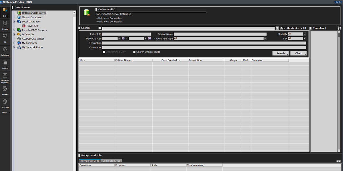
Our Dynamic Light Box is a simple image viewer to browse through slice images easily and quickly. This module provides axial, sagittal and coronal views and provides functions such as an Oblique Slice View, 3D Zoom and virtual endoscopy.
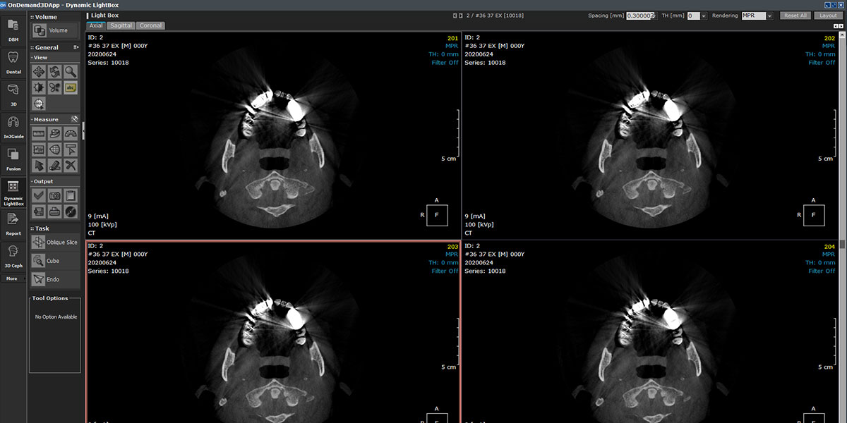
Our Report module keeps track of captured images and allows users to create quick reports in HTML format. The Report module supports the DICOM extended functions of capture, save, convert and print. Send captured images to PACS Servers or print on film, all fromthis module.
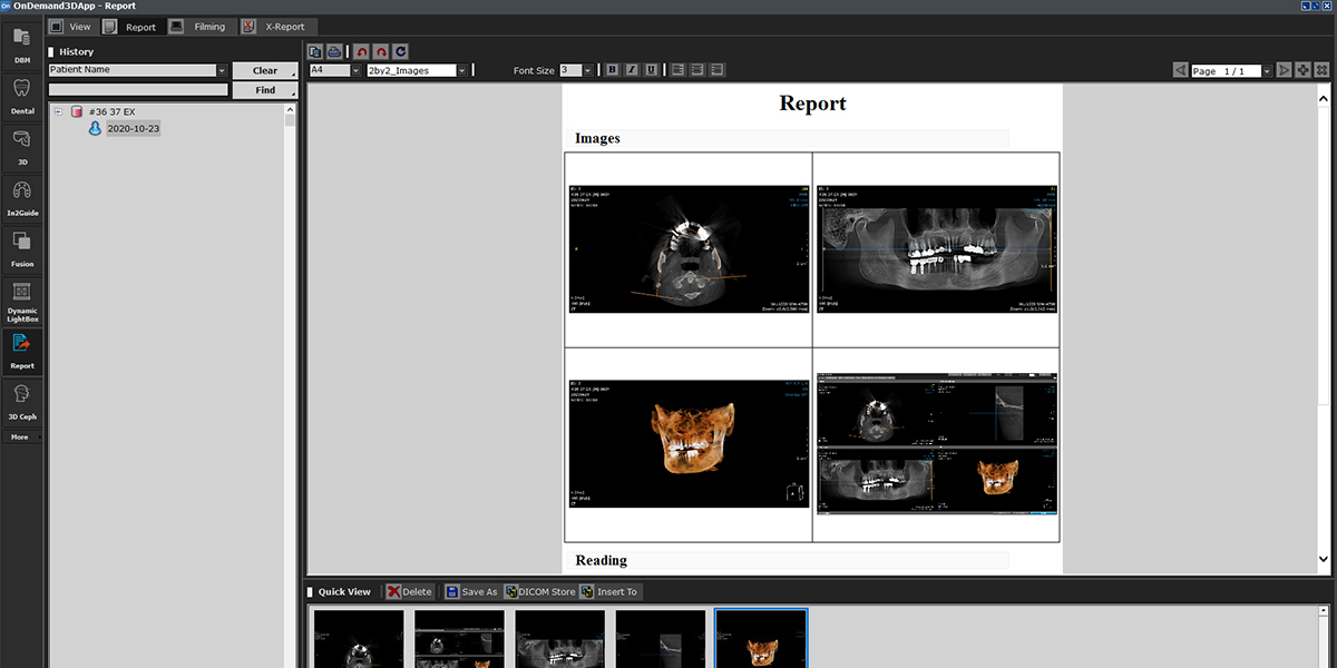
Our 3D module providesstate of the art tools for 3D visualization, segmentation, and analysis of DICOM images. The 3D module has various rendering modes such as VR (Volume Rendering), MIP, minIP, and X-ray. After segmentation, users will be able to export objects as STL data.
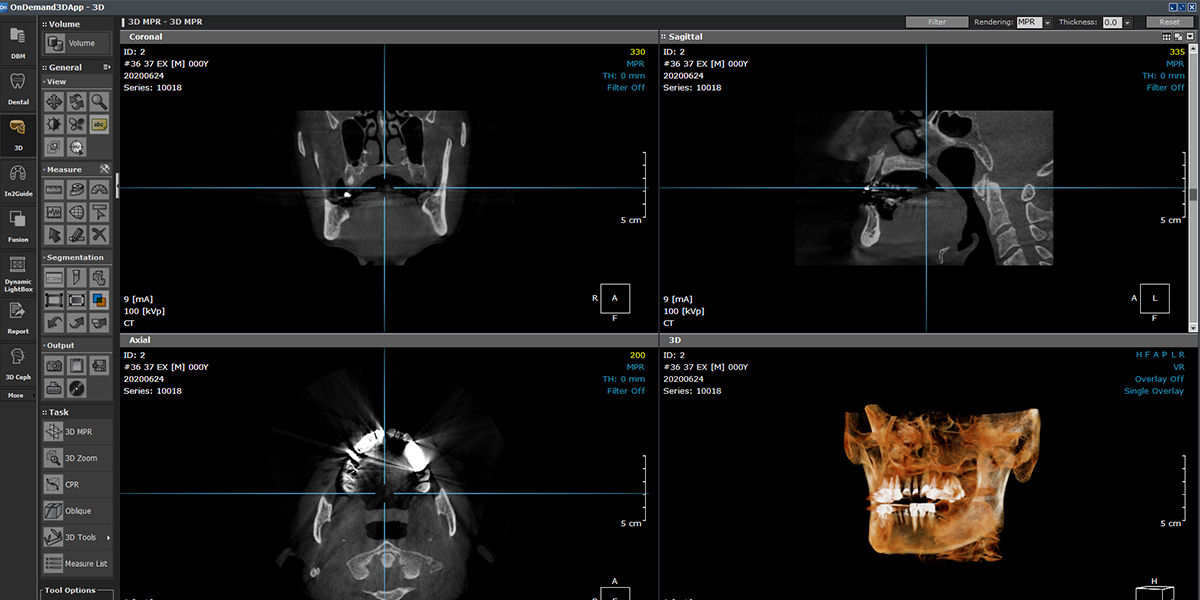
Our Dental module has all of the handy tools used for diagnosis and treatment planning including implant planning with real-size implant fixtures from major manufacturers complete with virtual teeth and every view format needed by dentists such as TMJ, bilateral TMJ, panoramic, and cross sectional views. Dental module also features 3D volume rendering, implant verification and MIP rendering functions.
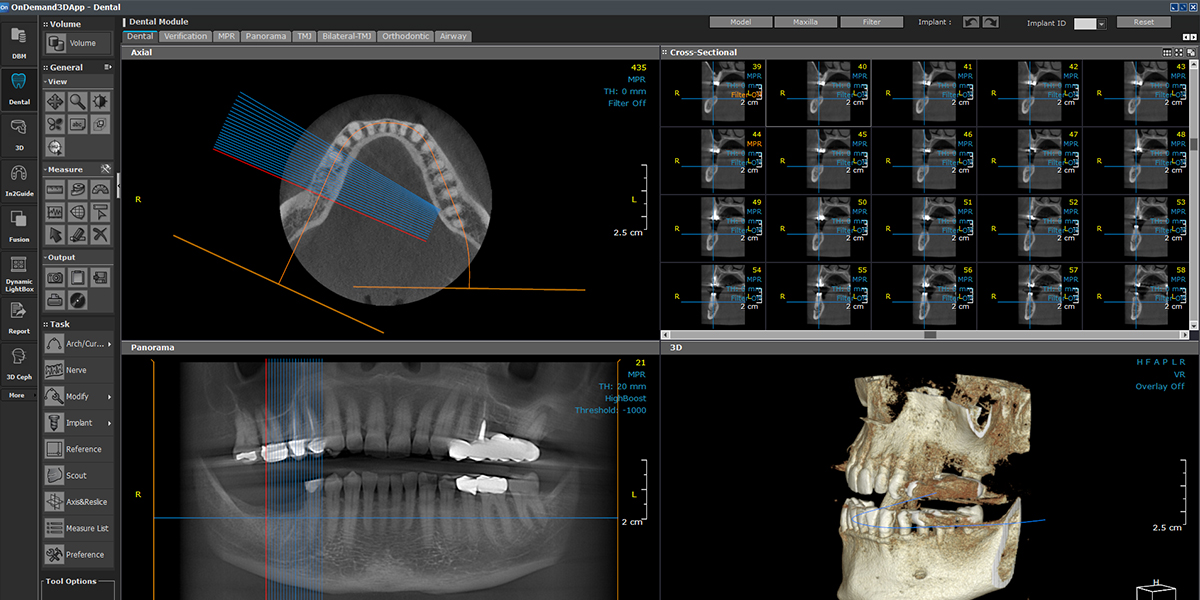
Our Fusion module is a visualization tool for superimposing two sets of DICOM data or for stitching two smaller FOV volumes to create a larger volume. Fusion uses the MI or Mutual Information method,a widely accepted technology for superimposition and stitching.
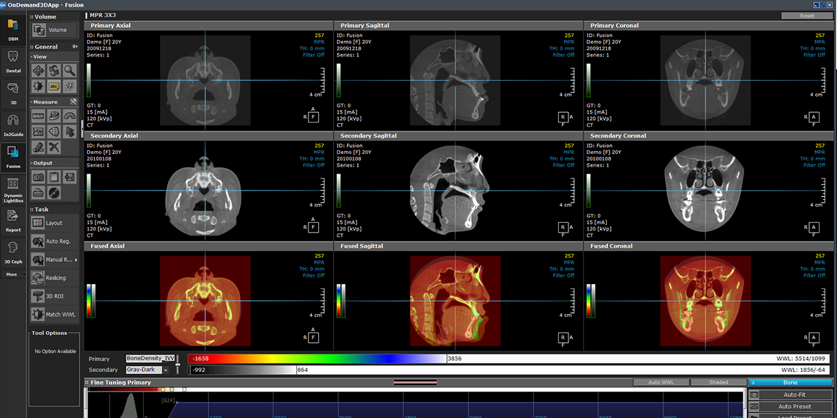
Our 3D Ceph calculates the relative functions between points, lines, and planes in a 3-dimensional setting providing more precise and accurate values for analysis. The user can customize and define the points, lines, planes, and functions for analysis, orthodontic and aesthetic treatment planning.
The user can also superimpose two sets of data, such as pre and post-op data for analysis, as well as use a 2D photo for a 3D volume mapping and generate a 2D X-ray for patient consultation.
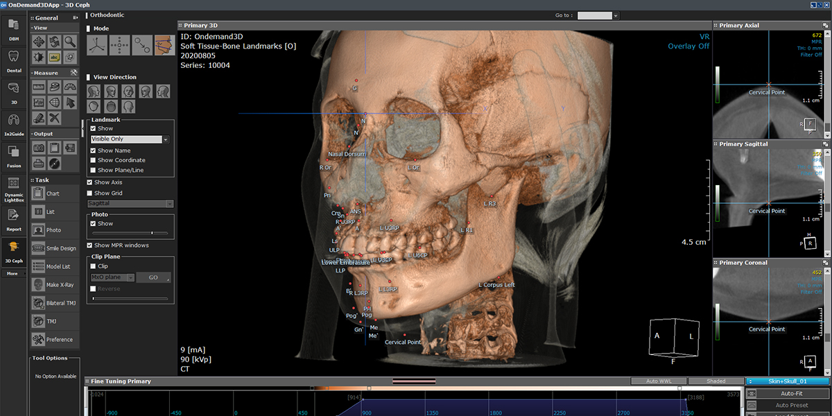
Our In2Guide utilizes OnDemand3D™’s powerful 3D engine to create a 3D volume from DICOM data for an intuitive way to plan your implant surgery. You can turn your virtual planning data into a real custom made surgical template with depth and angle control by ordering directly from In2Guide.
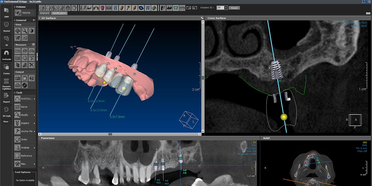
OnDemand3D™ takes integrated database management to a new level with our XImage. Both 2D and 3D dataare integrated into a modality-centered layout with full acquisition capabilities. A powerful tool that converts imported common image files into DICOM format (.dcm) for transmitting to PACS.XImage includes a selection of customizable Filter Presets along with a set of image manipulation and measurement tools.
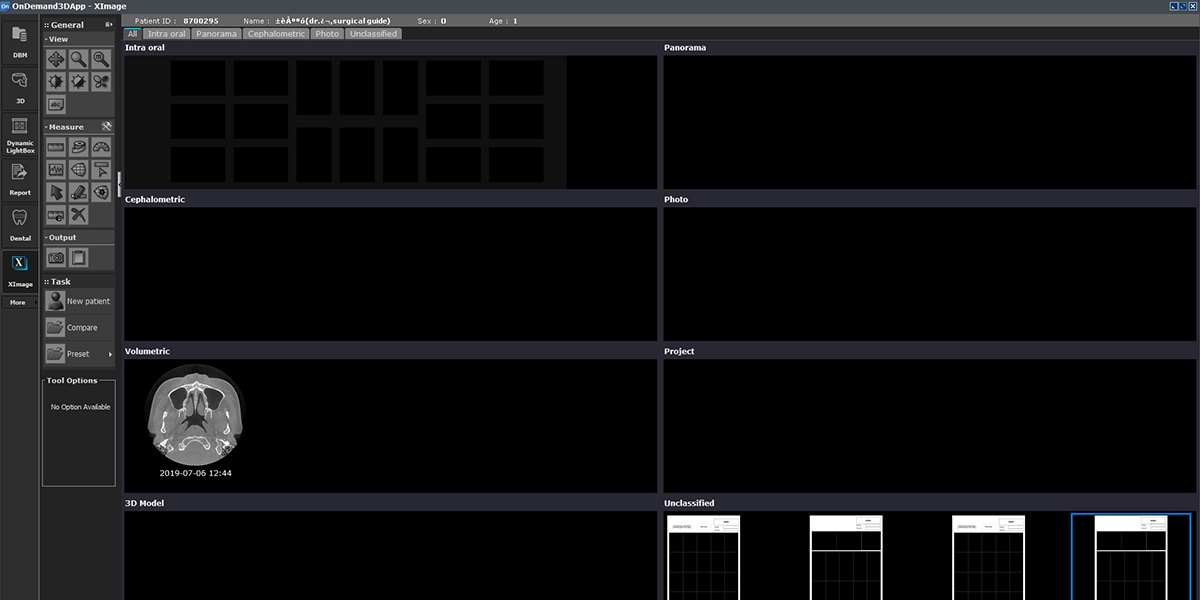
Our X-Report has two main features: the X-Report tool, included in most of the modules on OnDemand3D™ and X-Report Template Designer. The X-Report tool is a user-friendly method of patient reporting, where users will be able to simply drag and drop images from their screen onto a pop-up report template that can then be expanded for further editing. X-Report Template Designer, on the other hand, creates report templates for OnDemand3D™.It allows users to create a specialized report specific to a patient’s needs and increase the efficiency of writing a report.
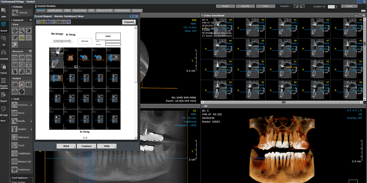
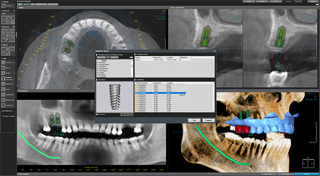
Planning Implant Placement
Implant surgery is one of the most complex and sophisticated areas. Through OnDemand3D, you can analyze the patient’s oral cavity in detail, place the implant in the right location, and perform a virtual operation.
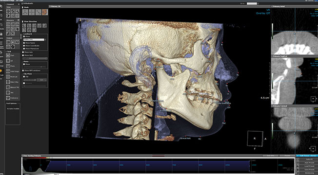
Orthodontics1
More than half of the world’s population have disproportionate teeth and maxilla. First, the 3D Ceph module allows you to plan and analyze a surgery or braces placement method. Because improvement in aesthetics is important as well as dental treatment, it helps to increase the trust between the dentist and the patient by showing and explaining the treatment process.
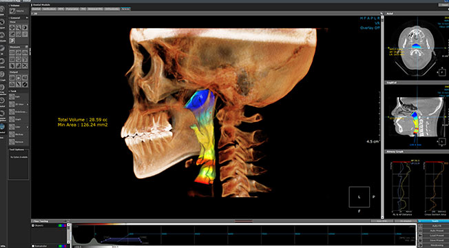
Airway Measurement
With just a few clicks, anyone in the dental field can easily and accurately measure airway volume. We are working hard on technology development so that we can measure more easily and accurately.
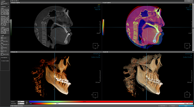
Comparative Analysis
It is very important to check the progress and difference of surgery. The OnDemand3D Fusion module visually shows the patient’s condition before and after surgery by superimposing two sets of dicom data, and sophisticated measurements can be performed through multiple options.
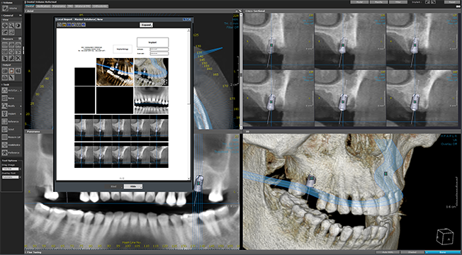
Analysis Report
For imaging centers, dental clinics, dental labs, and educational institutions, there are many advantages to analyze and shared patients’ CT results. You can highlight the patient’s diagnosis and treatment, and create a customized report.
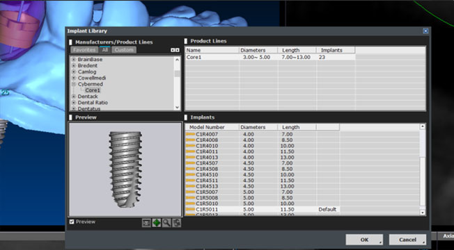
Implant Library
We have implant libraries from major implant manufacturers around the world, so you can plan and simulate realistic implant surgery. In addition, an implant library can be added.
Package
OnDemand3D™ App is a highly-advanced 3D imaging software developed for dentists, clinicians and research experts for use in the planning and simulation of patient treatment, accurate diagnosis, and advanced research. OnDemand3D™ utilizes DICOM data across modalities to reconstruct 3D volumes by means of the latest and best in 3D technology. OnDemand3D™ App provides specialized layouts, reconstructed images and tools for accurate and precise diagnoses.
It is composed of various modules according to the purpose of diagnosis and treatment of the user.
-
OnDemand3D Full Application
DBM, DLB, Report,
3D, Dental -
OnDemand3D-Dental
DBM, DLB, Report
Dental -
OnDemand3D-Server
Application, Server,
Project Viewer -
Add-on
Fusion, 3D Ceph, In2Guide,
X-Image, X-Report
OnDemand3D is a product used by major universities and dentists around the world.
It has been providing for over 20 years. During this long time, we have won a lot of trust and love from our customers.
We will provide more varied and innovative dental services.