
Важно! Перед началом скачивания и установки необходимо ОТКЛЮЧИТЬ АНТИВИРУС, иначе кейген может быть удалён.
Open Sound Meter на русском (iPad) скачать
Open Sound Meter на русском (MacOS 10.13 — 11.1) скачать [32 MB]
Open Sound Meter на русском (Windows 7 и выше) скачать [40 MB]
Open Sound Meter на русском (Linux-AppImage1) скачать [60 MB]
Видео-инструкция по установке и активации Open Sound Meter
Если видео не работает, обновите страницу или сообщите об этом в комментариях, поправлю.
Ссылка на видео: https://disk.yandex.ru/i/e3EOarqyvPvqcQ
Доброго дня!
Ну каждый же знает, что Umik и Smaart несовместимы )))
Они оба совместимы с автомобилем. но не одновременно. Так было ранее.
Кстати, если для Вас всё это не очевидно, то значит вы здоровы, и дальше пост может показаться странным.
А в нём речь пойдет о двух вещах, связанных с настройкой звука в авто:
1) о виртуальном Loopback на Mac os, позволяющем делать измерения в реальном времени без дуплесной звуковой карты.
2) о прикольной альтернативе Smaart, о которой только вчера подсказал мне добрый драйвовчанин kostik039 — Open Sound Meter.
Все на примере mac os правда. но думаю на винде тоже не сложно похожее замутить.
Начну с первого — Виртуальная (софтовая) обратная связь.
Хоть в Smaart, хоть в OSM, без обратной связи (loopback), невозможно измерить фчх в реальном времени.
Но обратная связь не обязательно должна быть аппаратная, можно использовать и софтовую, особенно если речь о простом стерео (как в почти всех авто).
Рецепт взят из области домашней звукозаписи и стримминга.
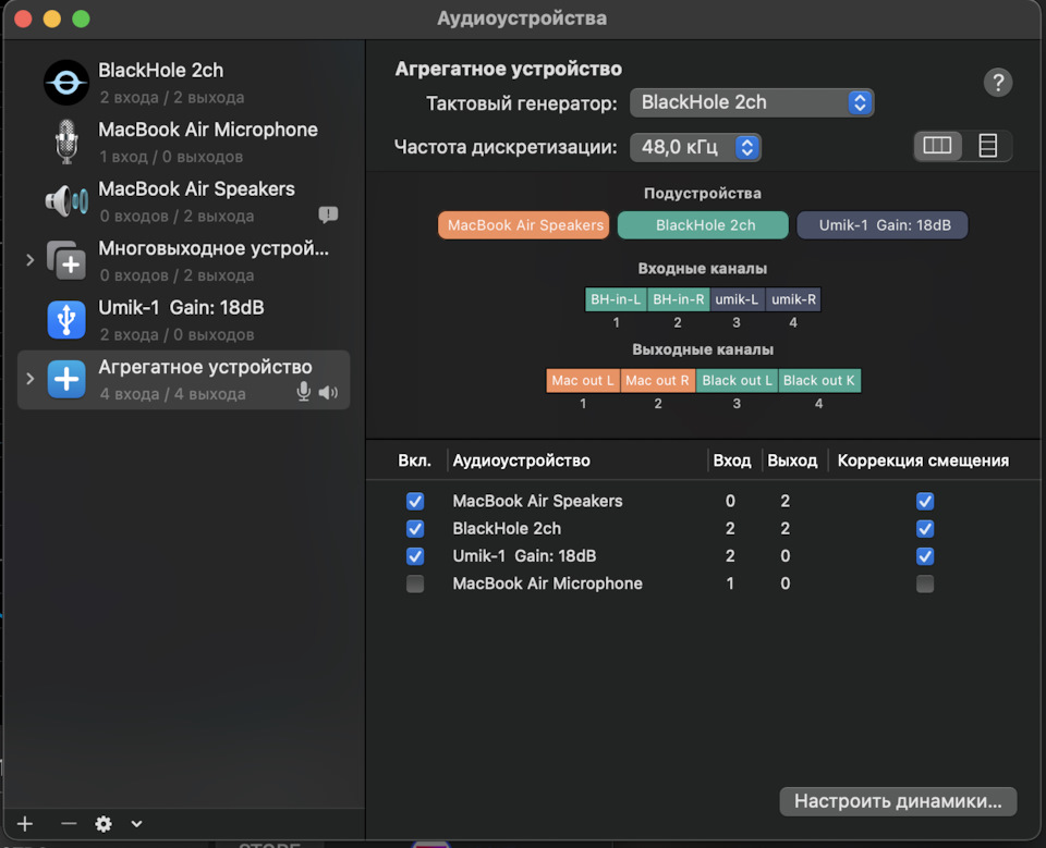
а) нужно поставить виртуальный аудиоинтерфейс. Я взял наиболее современный вариант для Mac = BlackHole. (Альтернатива = SoundFlower). Его достаточно просто поставить и всё, тут ноль настроек.
б) во встроенной в мак системной утилите «Настройка audio-Midi», нужно создать новое агрегатное устройство, и сконфигурировать его вот так:
* важна очерёдность аудиоустройств.
** первое устройство надо заменить на то, которое подаёт звук на ваш процессор)
*** это агрегированное устройство нужно пометить с помощью шестерёнки внизу экрана — Использовать для ввода и вывода звука.
**** обратите внимание, я переименовал названия каналов, без этого сложно потом разобраться.
в) далее в программе изменений (смаарт / osm) используем это агрегатное устройство
— в выводе с генераторав качестве aux.
— на входе в измерении (input) в качестве второго канала.
Что может быть проще ))
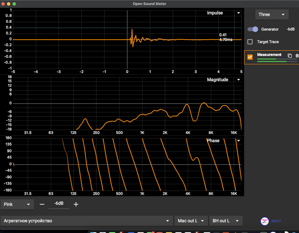
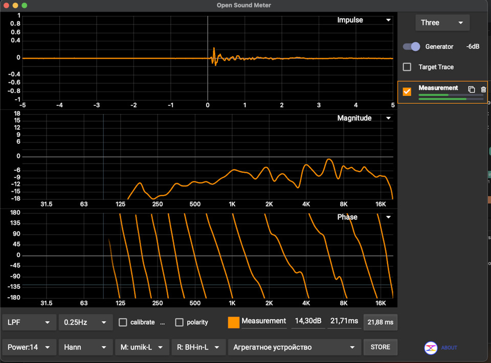
Больше никаких бесячих проводов.
Вторая часть поста.
Второй день нахожусь в хорошем настроении от новости, что у smaart появилась очень крутая альтернатива от российского разработчика: Open Sound Meter (opensoundmeter.com)
Это кроссплатформный бесплатный софт, для авто полностью покрывающий функционал smaart, и при этом в очень простом и удобном интерфейсе. Я бы не так сильно радовался, если бы не то, что на новых маках смаарт с торрентов вообще перестал работать. А тут не просто замена, но еще и улучшение в виде бонуса.
Правда сначала непривычно, и кажется, что функционал сильно урезан, но нет, просто настройки очень органично встроены в интерфейс.
Кстати, появившаяся версия для iPad уже имеет встроенный софтовый loopback, не требующий этих настроек.
Обзор на ютьюб:
Если бы например Резолют встроили этот софт в свой настроечный, представляю, насколько упростился бы процесс настройки…
Всем удачных настроек!
UPD
вот прикольный пост-сравнение.
www.caraudiojunkies.com/s…ter-RTA-Phase-ETC-Program
В стандарте замера АЧХ измерительный микрофон устанавливается на расстоянии 1м. На оси твиттера. Почему с одного метра? А почему бы и нет. Цифра ровная. Скажите спасибо, что мы используем метрическую систему. Почему на оси твиттера… Иначе привязать стандарт больше не к чему.
Стандарт подразумевает замер АЧХ под углами 30 и 60 градусов по горизонтали, на оси твиттера. Теоретически это вроде как бы, должно показывать, как будет себя вести АЧХ при перемещении слушателя в пространстве комнаты. Но в реальной ситуации, когда слушатель перемещается в пространстве все эти замеры не имеют особого смысла.
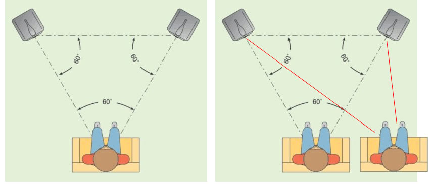
При перемещении слушателя даже на небольшое расстояние от центра, проходят несколько событий. Действительность гораздо более многогранна, чем одна АС на расстоянии 1 метра на оси твиттера.
Более типична ситуация, когда расположение ушей слушателей находится выше или ниже оси твиттеров. Но замеров АЧХ при смещении оси твиттеров вверх и низ не делают. Так как подобные замеры покажут катастрофическое искажения АЧХ почти у любой акустики. Вплоть до уровней +-20Дб.
Удобно замерять АЧХ одной АС. Но акустических систем обычно две. И АЧХ двух АС сильно отличается от АЧХ одной. Так расстояния от правой и левой АС и ушами слушателя не бывает одинаковым. А уже на частоте 3 кГц разница в расстоянии от левой и правой АС всего в 11 см. приводит к противофазности звучания каналов на высоких частотах.
Кардинально меняется угол входа звуковых волн в ушную раковину. Вы можете самостоятельно проделать простейший эксперимент. Взять легкую колонку и послушать ее звучание при различном угле относительно вашей ушной раковины. Покрутив ее вокруг уха и головы. Этот опыт вам сразу покажет, что наилучшая фокусировка звуковых волн происходит под углом около 15 градусов. А совсем не по правилам равностороннего треугольника.
Человек слышит в основном вперед, а не в сторону. Причем разница в звучании (АЧХ) от угла входа звуковых волн в ушную раковину будет радикальной. На слух, АЧХ от различного угла входа в ушную раковину меняется на значения порядка +-25Дб.
И никто не знает, каким должен быть «правильным» угол входа в ушную раковину. Этот вопрос находится вне дискурса.
Замеры отдельных динамических головок, и их АЧХ с одного метра, на оси динамика имеют огромный смысл. Таким образом понятно, какие характеристики этот динамик имеет. И как его лучше использовать.
В случаи когда производятся замеры готовых акустических систем, измеряют, то что удобно измерять. С целью публикации красивых графиков в рекламных материалах. Никаких особовых выводов и смыслов из этих графиков получить нельзя.
Предлагаем вам использовать практически работающую технологию замера АЧХ. Ее повсеместно используют в профессиональной деятельности, в концертной практике, для отстройки звучания акустики в различных помещениях.
В реальной жизни не важно, какая у одной колонки АЧХ на расстоянии 1 м. на оси твиттера. Так как в реальной жизненной практике так не бывает, — никто не слушает одну колонку с расстояния в 1м.
Важно другое. Как акустическая пара формирует общую картину АЧХ в 3D пространстве.
Для этой цели удобна программа — Анализатор аудио спектра TrueRTA. Но может быть любая другая программа анализатор спектра с большой разрядность (1/24 октавной полосы).
Сглаживание в 1/3 и 1/6 октавной полосы, как это принято делать в статьях для рекламы акустики, в большенстве случаев будет мало. Заведомое снижение разрешения в 3-6 раза, разумется делает гафик более ровным. Но на этом разрешени пропадают узкие выбросы АЧХ.
Которые лучше увидеть, и занать, что они есть. Или занатать, что их нет.
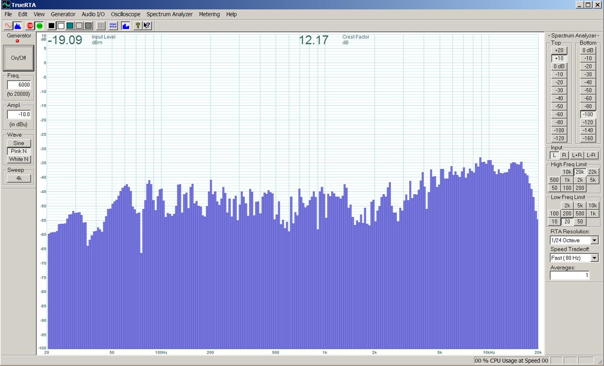
Проще всего использовать ее на ноутбуке. Но имейте ввиду, что процессора уровня Atom ей будет недостаточно, для того, что бы считать 1/24 октавной полосы в реальном времени. Нужен процессор хотя бы уровня нижнего i3.
При наличии длинного микрофонного кабеля, в домашних условиях пойдет и ПК. Менее удобно, но если зрение или очки хорошие, работать вполне можно.
Потребуется измерительный микрофон и источник фантомного питания для него. Так как все измерительные микрофоны конденсаторного типа. И требуют для своей работы питания.
Фантомное питание есть в большинстве нормальных звуковых карт. И как правило, звуковая карта с фантомным питанием стоит так же, как и без фантомного питания. Даже если вам сейчас не нужно мерить АЧХ, — покупайте карточку с фантомным питанием. Возможно через 5-10 лет оно вам пригодиться. Про звуковые карты можно почитать — Звуковые карты usb, полный обзор.
При этом эти микрофоны можно использовать как обычные качественные микрофоны для записи чего угодно. Это не есть выброшенные разово деньги на замер АЧХ. Они как микрофоны вполне себе приличные. Лично записал несколько сотен часов закадрового текста для ТВ программ. Они лучше чем топовые петличные микрофоны класса Сони-Синхайзер под $500 (у них диафрагма больше, чем у петличных микрофонов).
А если энтузиазм по азмеру АЧХ у вас совсем исякнет — измерительные микрофоны хорошо ликвидны на авито.
Производитель прикладывает график АЧХ микрофонов:
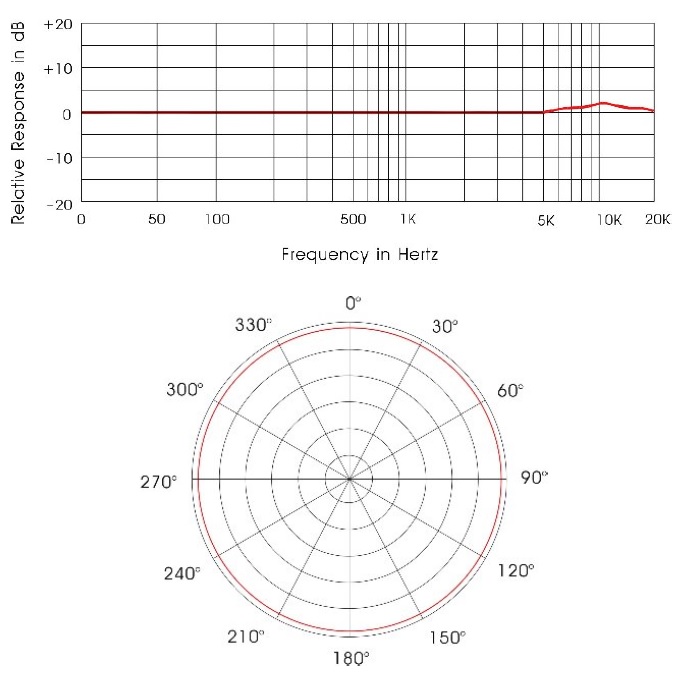
В большинстве случаев этот график АЧХ будет иметь очень близкое соответствие. В измерительных микрофонах очень модно использовать капсюли WM-60A Panasonic.
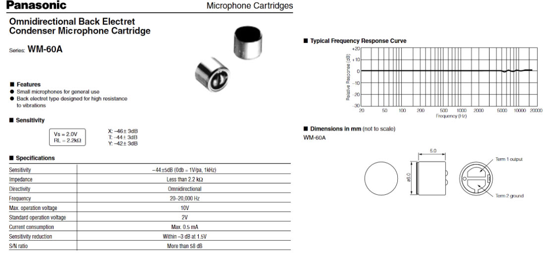
Стоят эти капсюли WM-60A в большой партии порядка 1 доллара.
Продают их китайцы по цене порядка 15 долларов — ссылка.
Производить микрофоны с ровной АЧХ, в современном мире, приблизительно так же сложно, как делать столы с ровной столешницей.
Для контроля анормальности АЧХ можно посмотреть, что он показывает на паре известных вам мониторов. Либо сравнить его с другим микрофоном, с известной АЧХ.
Все очень просто. Программа генерирует розовый шум. Акустика его воспроизводит. Перемещая измерительный микрофон мы смотрим, в реальном времени, общую картину АЧХ в пространстве. Получается очень быстро. И очень информативно.
За пару минут можно отсканировать все. Любые углы. Любые расстояния. Пройти всю комнату.
Измерять же АЧХ смартфоном, используя микрофон самого смартфона, занятие абсолютно бестолковое. Ничего вы не замерите, — даже приблизительно понять какая АЧХ не получится. Не тратьте на это время.
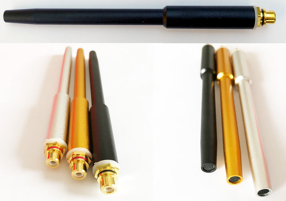
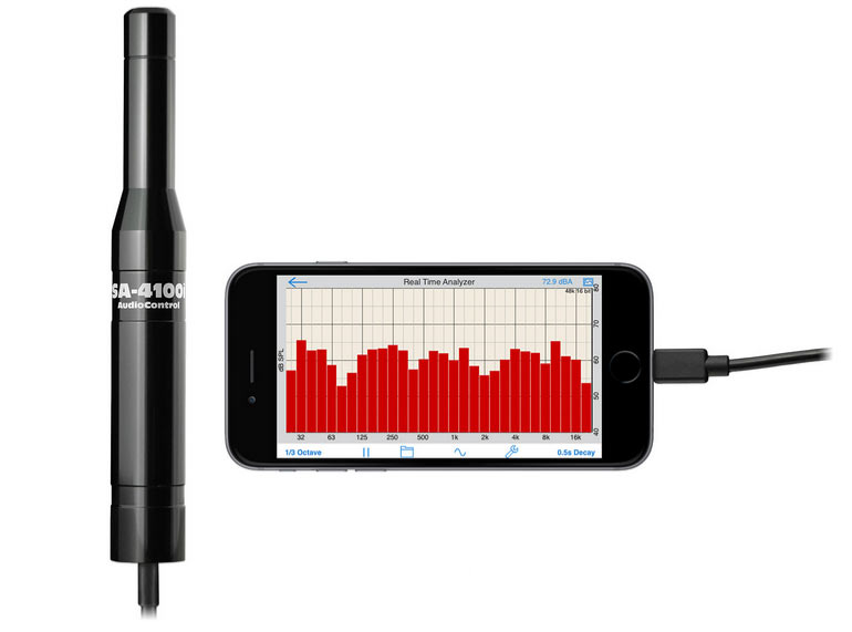
Существуют приблуды для смартфонов. Например для iPhone (не всех версий!) есть SA-4100i. Но это мы не рекомендуем. Будет менее удобно и как это всегда у смартфонов, — все сильно упрошено и опошлено.
Мы нашли дивайс для замера не только АЧХ, но и АЧХ наушников Dayton Audio iMM-6. То же под iPhone:
Если кто знает подобные устройства под андроид — напишите в коментах.
Следует понимать, что не следует ставить себя задачу свести акустику с идеальной АЧХ.
Ровная, красивая АЧХ получиться только в том случаи, когда на НЧ/СЧ динамике будет стоять «жесткий» фильтр в районе 2.5 кГц, или еще ниже.
И ровная эта АЧХ будет только в самом их ближнем поле. После того как вы походите с микрофоном по комнате, и увидите реальную АЧХ в пространстве комнаты, желание прибывать или убавить 2Дб в каком то месте у вас сразу исчезнет. К примеру, вы сразу обнаружите, что ВЧ на расстоянии одного метра вполне достаточно. Но если мерить эти ВЧ уже с расстояния 2-3 метра, — они по дороге куда-то сильно деваются.
«Жесткий» фильтр в районе 1.5-2.5 кГц задает специфический «характер звучания» акустики. Его можно охарактеризовать, как типичный «новодел» или «мониторное» звучание. Годится слушать скрипки и аудиофильский джаз и прочею Реббеку Пупкину. А слушать музыку будет на этой акустике не особо приятно.
АЧХ конечно должна пребывать в неких рамках. На практике даже меньших чем чем это декларирует стандарт DIN (+-3Дб).
Воспринимаемое людьми качество не имеет прямой зависимости от ровности АЧХ.
Если вы сталкиваетесь с АС у которой АЧХ имеет идеальную форму близкую к линии, вероятность того что на этой акустике будет приятно слушать музыку (не демо фонограммы) будет стремится к нулю.
80 полосный цифровой эквалайзер, которым можно сделать идеально-плоскую АЧХ, не поднимает класс акустических систем.
Если вам требуется точно померить АЧХ… Увидеть, как она выглядит во всех нюансах, то рекомендуем программу:
Arta Software
От всех других аналогичных программ ее отделяет интуитивно понятный интерфейс при огромном функционале возможностей.
Последняя версия программы доступна на сайте разработчиков. Ниже, в разделе приложение, мы даем ее полное описание и методику работы с программой Arta Software. Программа вроде платная. Но это мало кого останавливает, так как, кто ищет тот всегда найдет.
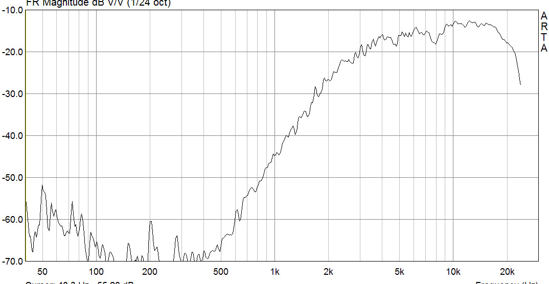
Измерять АЧХ можно самым простейшим образом. Тупо послал сигнал на усилитель-динамик и замерил микрофоном результат:
АЧХ почти сразу можно увидеть в таком виде:
Помимо этого программа позволяет замерять всякие другие разные полезности. Кто желает глубоко погрузиться в тему, — изучайте приложение. Но имейте ввиду, в бытовой, слушательской практике, такие точные измерения не несут ни какого смысла. А вот для разработчиков аудиосистем программа Arta Software очень весьма полезная и даже необходимая.
Ниже мы приводим полное руководство по работе с программой Arta Software.
Рекомендуем для прочтения:
«Характер звучания» акустики
Почему в акустике не работает принцип «ксерокса»
Приложение. (TrueRTA и Arta Software)
Описание TrueRTA.
Анализатор аудио спектра TrueRTA, работает в режиме реального времени, отлично подходит для настройки амплитудно-частотных характеристик акустических систем в различных помещениях и залах. Программное обеспечение включает в себя целый набор инструментов, в частности, спектральный анализатор реального времени (Real Time Analyzer), двойной осциллограф, генератор сигналов, цифровой измеритель уровня и коэффициента амплитуды сигнала или крест-фактора. Интерфейс приложения крайне прост и удобен, все настройки могут быть развернуты в виде панелей на основном рабочем окне.
Программное обеспечение предоставляет возможность самостоятельно настраивать масштабы, параметры и диапазоны звуковых измерений, проводит обработку и усреднение входных данных, имеет функцию фиксации пиков. Сигнал на экране осциллографа может быть остановлен в любой момент времени и прокручен в разные стороны. Также предлагается пять различных цветовых схем для графической области окна.
Полученные с помощью TrueRTA измерения позволяют детально и «на лету» оценить акустику, определить нелинейные искажения, проверить правильность расчетов разделительных фильтров. Максимальное разрешение достигает 1/24 октавной полосы. Программа позволяет выявить не только спектральный состав гармоник, но и просчитать коэффициент нелинейных искажений для каждой из них. Расчет уровня гармоник в приложении необходимо проводить вручную.
Кроме того программа TrueRTA может генерировать аудио сигналы любой частоты (в пределах от 1 до 22000 Гц) и амплитуды. Приложение позволяет проводить замеры белым шумом, розовым шумом (стандартным для акустических измерений) или синусоидальным сигналом. Результаты измерений можно распечатать или сохранить в ячейках памяти, а затем сравнить между собой. Последние версии софта имеют возможность определять импульсные характеристики звуковых сигналов.
Описание Arta Software.
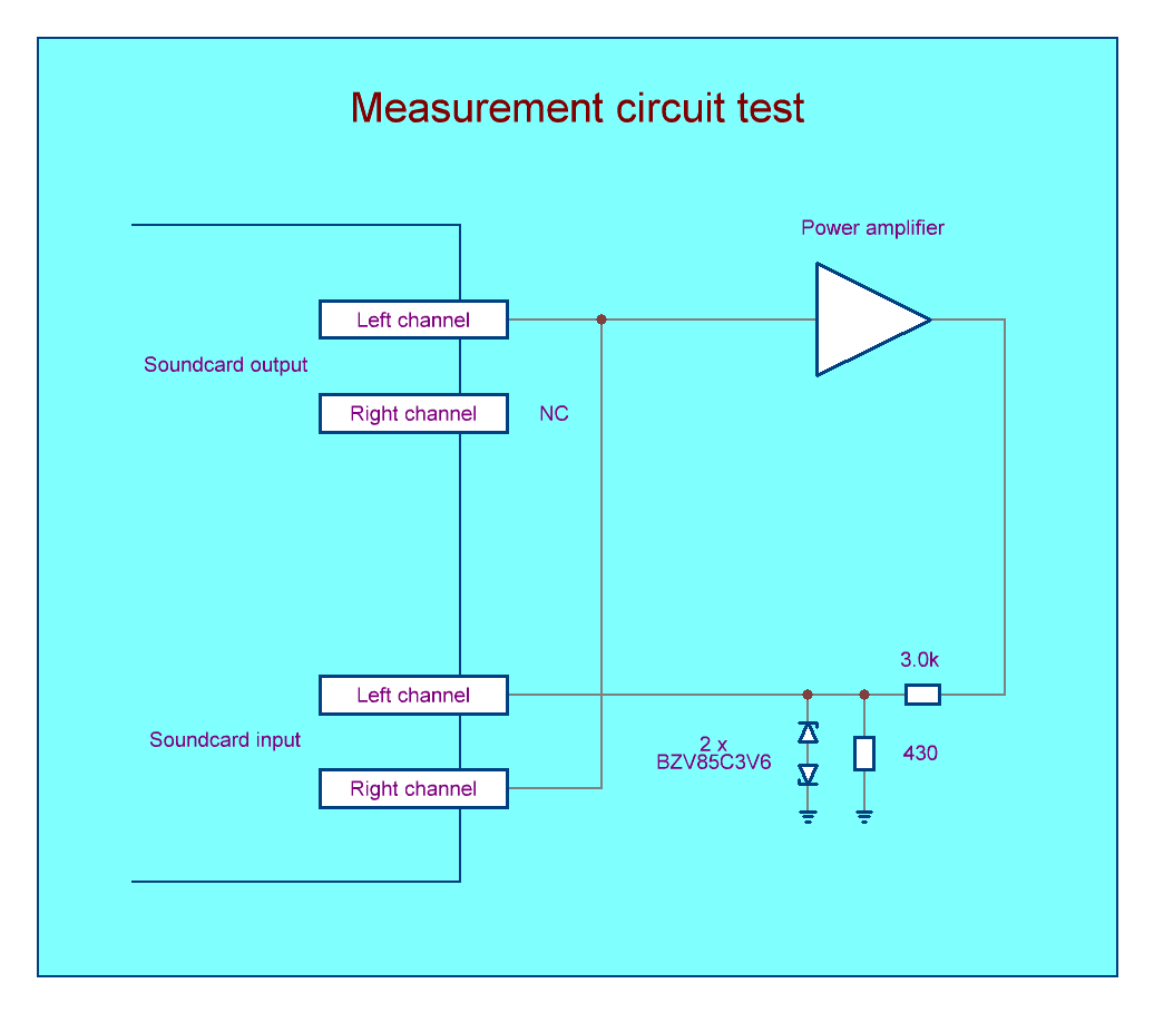
Проверка измерительного тракта.
Перед началом непосредственно измерений необходимо удостовериться, что используемый измерительный тракт обладает достаточной линейностью. Для этого производится подключение оборудования по схеме.
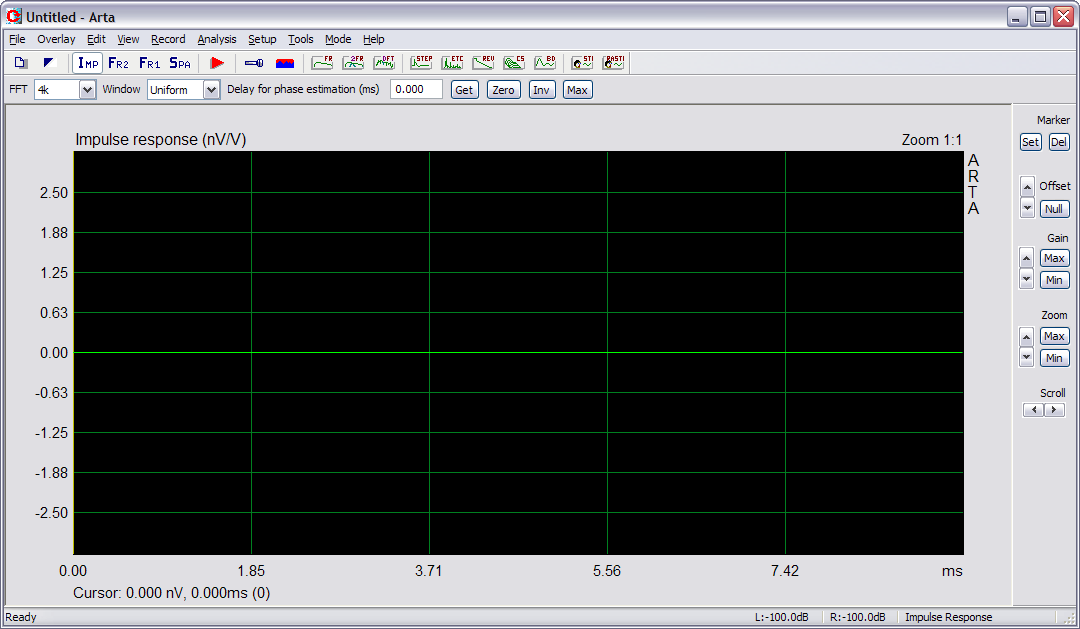
Запускаем Arta. Откроется окно, называемое окном импульсной характеристики (Impulse Response).
Стандартный темный интерфейс можно поменять на светлый с помощью функции меню Edit – B/W background color. Также я изменяю стандартную цветовую гамму через меню Edit – Colors and grid style.
Первым делом производится настройка программы. Для этого переходим в меню Setup – Audio devices.
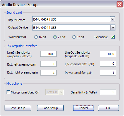
В полях Input Device и Output Device указывается используемая звуковая карта. В поле WaveFormat выбирается разрядность цифровых данных, с которыми будет работать звуковая карта. Разработчики Arta Software рекомендуют использовать 24 или 32 bit, но только в том случае, если используемая звуковая карта является высококачественной. Мотивируют это справедливо – далеко не все звуковые карты, предназначенные для работы с разрядностью данных 24 bit, обладают линейностью на уровне хотя бы 16 bit. Также возможно появление сообщения об ошибке при запуске измерений, если звуковая карта не поддерживает указанную в поле WaveFormat разрядность. При выборе 24 либо 32 bit автоматически устанавливается галочка Extensible. Снимать ее не нужно, иначе при запуске измерений программа выдаст ошибку. Все остальные поля предназначены для работы с калиброванным измерительным комплексом, поэтому я их пропускаю. Выполняем установки и нажимаем ОК.
Переходим в меню Setup – Calibrate devices
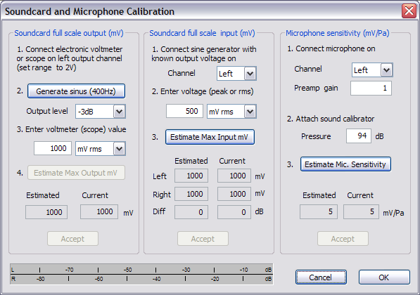
Это меню предназначено для калибровки измерительного комплекса. Нас интересует только раздел Soundcard full scale output (mV). Здесь нажимаем кнопку Generate sinus (400Hz) и устанавливаем на выходе усилителя необходимое для теста напряжение. Никаких критических требований к величине этого напряжения нет, просто устанавливается не большая и не маленькая величина. Я установил по вольтметру 0.7041 v. Обратите внимание, что в поле Output level установлено значение -3 dB. После установки нажимаем повторно кнопку (теперь уже с надписью Stop Generator) и закрываем окно.
Переходим в меню Setup – Analysis parameters
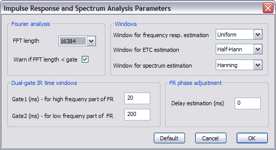
Здесь все установки нам подходят, за исключением FFT length. Это значение необходимо изменить на 16384. Именно такое, поскольку в дальнейшем при измерениях я буду использовать количество сэмплов тестового сигнала – 16384. Когда потребуется сменить (при измерениях зависимости нелинейных искажений от частоты), я об этом упомяну. Вообще, желательно, чтобы размер FFT всегда совпадал с количеством сэмплов тестового сигнала.
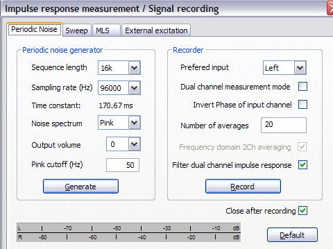
Переходим в меню Record – Impulse response/Signal time record (6). Выбираем вкладку Periodic Noise, если она не выбрана.
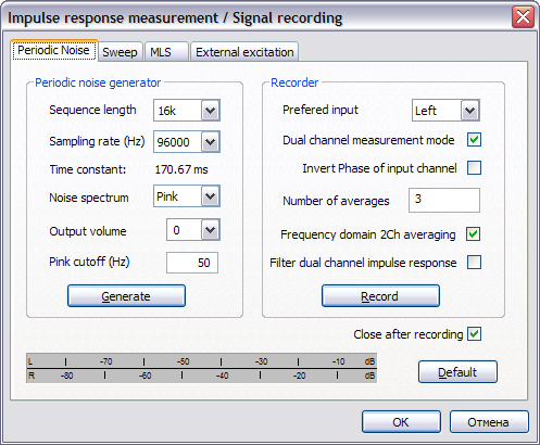
Здесь, в поле Sequence length (количество сэмплов на период тестового сигнала), устанавливаем значение 16k (16384). При использовании частоты дискретизации 96 kHz, период составляет 16384/96000 = 170.67 ms, что в 3.4 раза больше значения, необходимого для измерения нижней границы звукового диапазона – 20 Гц. Увеличивать период, значит не только расширение полосы частот вниз, но и увеличение разрешения по частоте. При акустических измерениях платой за это выступает насыщение измеренного сигнала поздними отражениями помещения. На остальных полях сейчас не буду заострять внимание, вернемся к ним позже, при непосредственно акустических измерениях. Пока производим установку параметров согласно изображению и нажимаем кнопку Generate. Внизу, на индикаторе уровня, отобразятся уровни входных сигналов. С помощью доступных регулировок чувствительности устанавливаем значения в диапазоне -20…-10 dB, после чего отключаем генерацию повторным нажатием кнопки. Теперь нажимаем кнопку Record. После завершения измерений окно закроется автоматически.
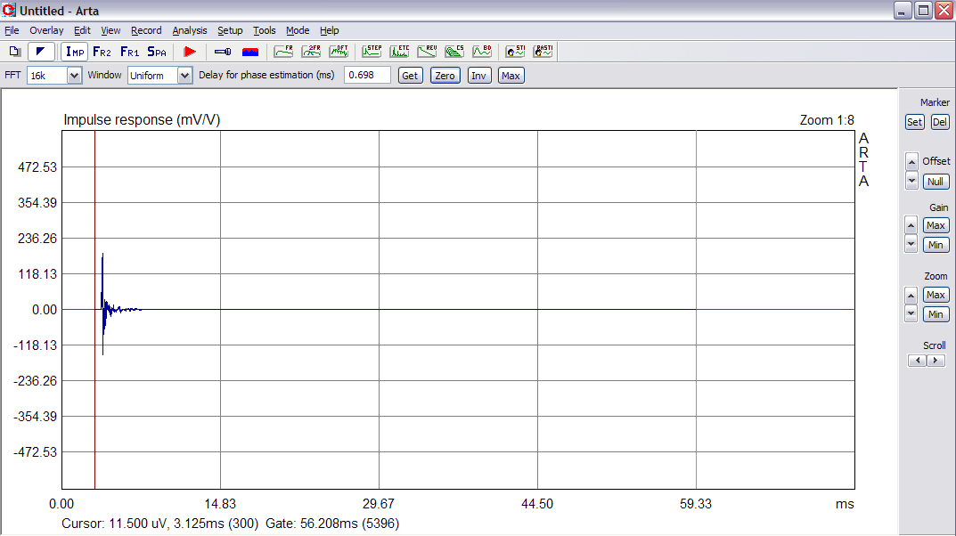
Если все прошло успешно, в окне импульсной характеристики должен наблюдаться импульсный отклик системы.
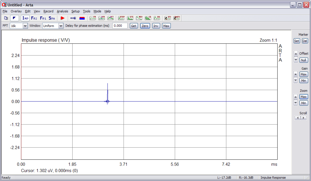
Для работы с окном импульсной характеристики в Arta используются курсор и маркер. Курсор устанавливается левой кнопкой мыши и определяет начало временнОго окна. Маркер устанавливается и удаляется правой кнопкой мыши и определяет конец временного окна. ВременнАя разница между положениями курсора и маркера – это окно измерений (Gate). Из информации, что находится внутри этого окна, производится расчет графиков АЧХ, ФЧХ, ГВЗ, кумулятивного спектра и графика распада. Остальные графики отображают результаты измерений на основе полного периода тестового сигнала. Внизу окна Impulse Response отображена позиция курсора, ей соответствует 0 ms, 0 сэмплов. В данном случае эта позиция и требуется. Для вычисления фазовой характеристики необходимо установить значение задержки от положения курсора до максимума импульса. С помощью расположенных справа кнопок Gain, Zoom и Scroll устанавливаем вид импульса так, чтобы были видны позиции сэмплов, после чего устанавливаем маркер в центр импульса и нажимаем на панели инструментов кнопку Get. В поле Delay for phase estimation (ms) должно отобразиться значение задержки.
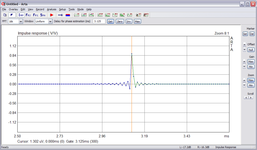
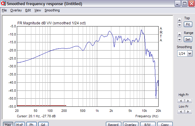
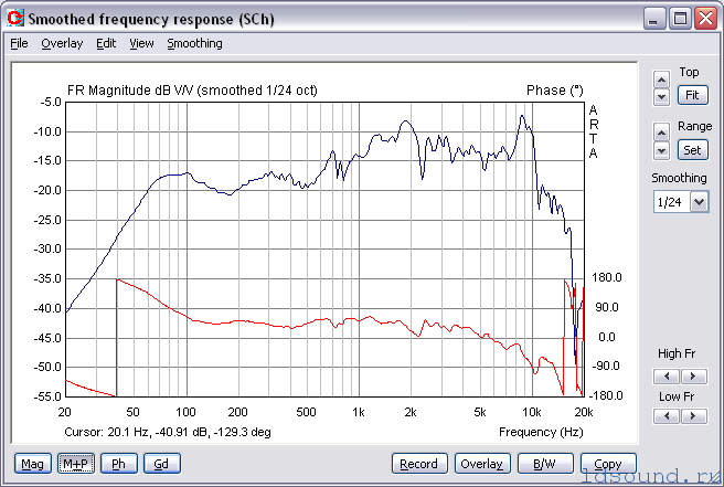
С помощью кнопки Zoom делаем видимым все окно измерений (170 ms) и устанавливаем маркер в самом его конце. У меня длина окна измерений (Gate) соответствует 170.469 ms (16365 сэмплов). Теперь можно просмотреть результаты измерений. Сейчас нас интересует только линейность АЧХ и ФЧХ, поэтому нажимаем на панели инструментов кнопку с буквами FR (либо через меню выбираем Analysis – Single-gated smoothed Frequency response/Spectrum). Откроется окно Smoothed frequency response.
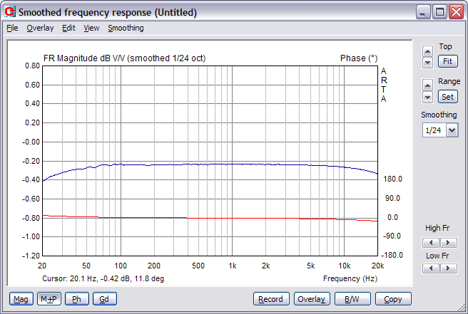
Слева внизу расположены четыре кнопки, – Mag, M+P, Ph и Gd. Они отвечает за отображение графиков соответственно АЧХ, АЧХ+ФЧХ, ФЧХ и ГВЗ. Справа на панели, в поле Smoothing, можно выбрать сглаживание графика. Левой кнопкой мыши на графике производится установка курсора, а правой – открываются свойства графика. Более подробно к этому, а также к ряду других возможностей, я вернусь позже. Сейчас же результат получен, и можно видеть полную пригодность измерительного тракта для проведения измерений импеданса и акустических измерений.
Пока есть результат измерений, можно самостоятельно ознакомиться с меню программы и просмотреть, как выглядят графики для системы, идеальной относительно динамиков. Например, переходная характеристика. Программа не умеет отправлять на принтер результаты измерений и не умеет экспортировать их в графический формат, но позволяет перенести в буфер обмена. Для этого в каждом окне доступна кнопка Copy (либо через меню Edit – Copy). Посленажатия откроется окно Copy to Clipboard.
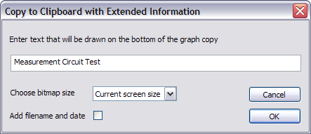
В текстовом поле можно написать любые комментарий к графику, а в поле Choose bitmap size выбрать из списка размер изображения. Галочка Add filename and date добавляет к графику имя файла импульсной характеристики и текущую дату. Для примера, результат показан ниже.
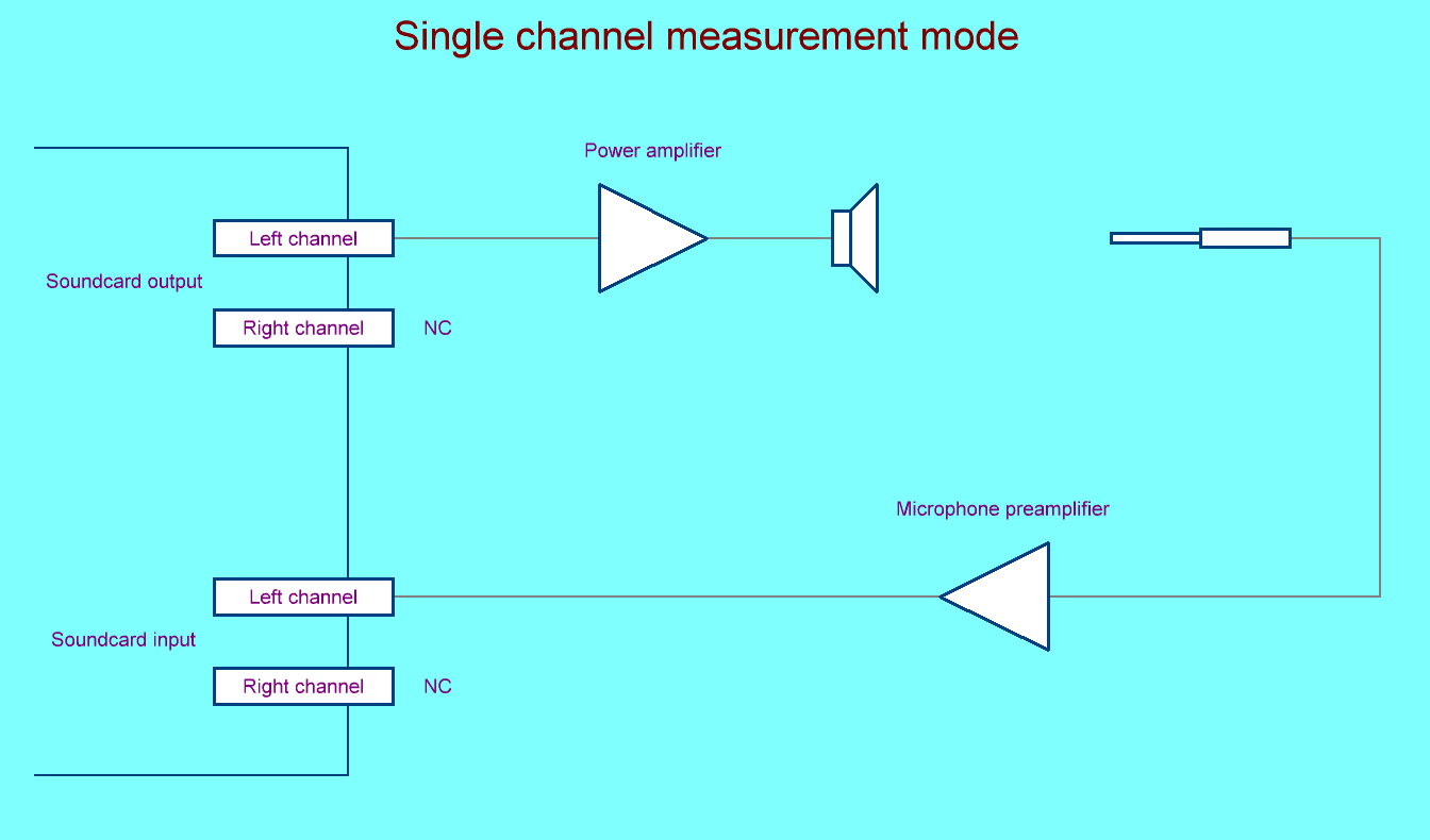
Для проведения акустических измерений возможно использовать одно или двухканальную схемы:
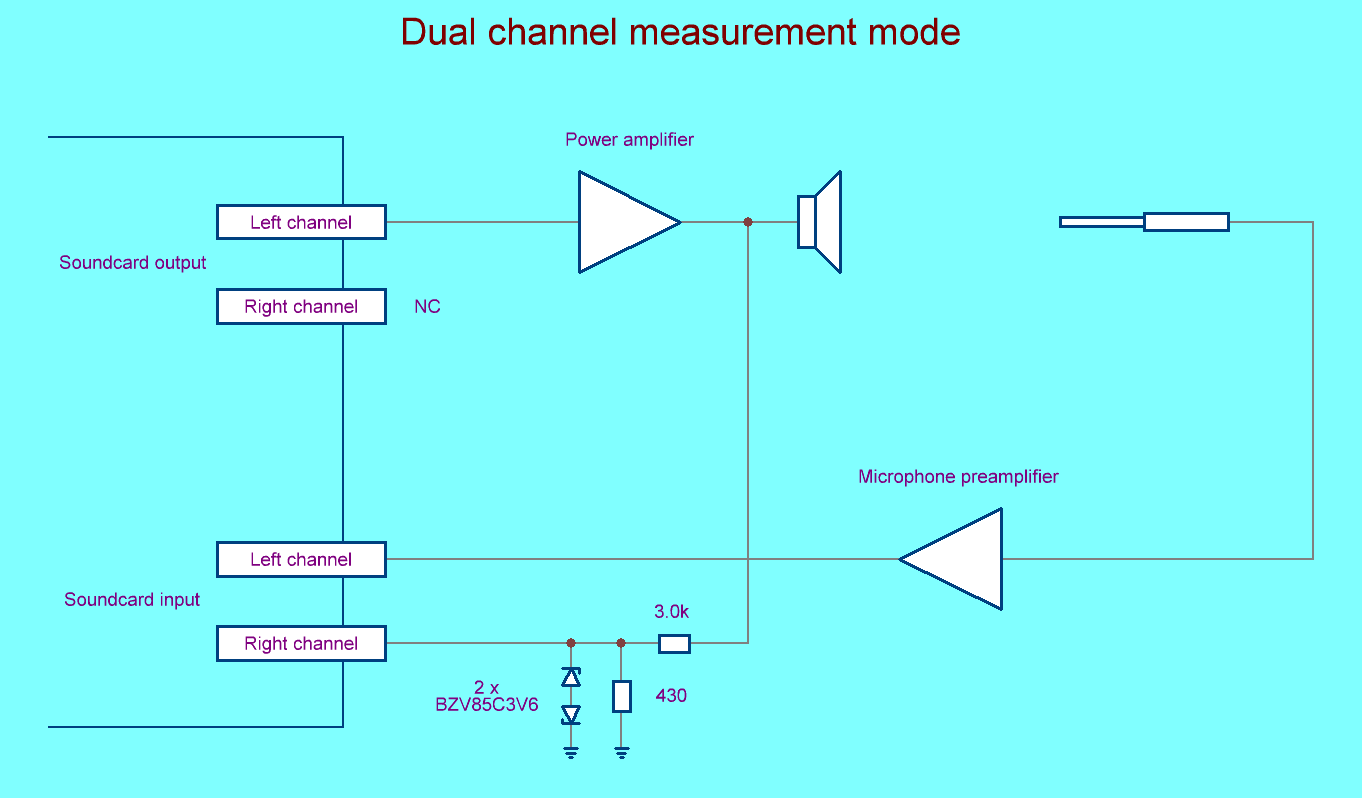
Рекомендуется работать с двухканальной схемой измерений, но в случае использования встроенного в звуковую карту предварительного усилителя для микрофона, подключенного к входу Line In, использовать двухканальную схему не получится.
Одноканальный же метод обладает недостатком – в Arta не определена опорная позиция курсора. Некоторое время я вынужден был использовать одноканальную схему измерений, поэтому пришлось искать метод определения этой позиции. Такой метод был найден. Возможно, он не самый лучший и не самый правильный, но другого метода найти не удалось. Детально об этом расскажу чуть позже. Сейчас же подключаем оборудование в соответствии с выбранной схемой измерений и располагаем перед измеряемым динамиком стойку с микрофоном. Для комплексных измерений динамиков для будущей акустической системы расстояние до микрофона следует выставлять одинаковым и в процессе измерений не производить изменение выходного напряжения усилителя.
Для измерений АС в дальнем поле, чтобы упростить процедуру установки микрофона строго на оси ВЧ излучателя, рекомендую использовать лазерную указку. По ходу написания материала я буду проводить измерение в ближнем поле (расстояние между микрофоном и динамиком составляет приблизительно 20 см) широкополосного динамика 4А28 без акустического оформления. Почему я не указываю точного значения напряжения на выходе усилителя и не придерживаюсь строгого расстояния между динамиком и микрофоном. Все просто. Для измерения абсолютных величин звукового давления требуется либо калиброванный измерительный микрофон, либо самостоятельное выполнение процедуры калибровки по динамику, на который есть результаты измерений, полученные с помощью калиброванного измерительного комплекса. Использовать как эталон значение чувствительности динамика, рассчитанное вместе с остальными параметрами Тиля-Смолла, нельзя. Это значение имеет слишком мало общего с реальной чувствительностью динамика, и тем более с его АЧХ. Придерживаться конкретной величины напряжения, подводимого к динамику, следует в том случае, когда проводится измерение зависимости нелинейных искажений от частоты.
Запускаем Arta. Откроется уже знакомое окно импульсной характеристики. Проверяем и при необходимости корректируем установки в меню Setup – Audio devices. С помощью генератора синусоидального сигнала 400 Hz, доступного через меню Setup – Calibrate devices, производим установку требуемого напряжения на выходе усилителя. Проверяем установки в меню Setup – Analysis parameters. Переходим в меню Record – Impulse response/Signal time record, открываем вкладку Periodic Noise. Это меню частично уже знакомо. В поле Sequence length производится установка количества сэмплов на период тестового сигнала, в поле Sampling rate (Hz) – частота дискретизации (Fs). В поле Noise spectrum выбирается тип периодического шумового сигнала: White (белый), Pink (розовый) и Speech (речевой). В поле Output volume устанавливается уровень тестового сигнала. Поле Pink cutoff (Hz) изменяет частоту среза при использовании розового шума. Справа, в поле Prefered input выбирается измерительный канал. В данном случае это канал, к которому подключен микрофон. В обеих схемах измерения (Figure 27 и Figure 28) в качестве измерительного используется левый (Left) канал. Установка галочки Dual channel measurement mode задействует двухканальный метод измерений. Галочка Invert phase of input channel служит для изменения фазы входного сигнала на 180 градусов. Это требуется, если подключение измеряемого динамика произведено с обратной полярностью.
В поле Number of averages указывается количество измерений, из которых методом усреднения будет рассчитана импульсная характеристика. При акустических измерениях рекомендую устанавливать число измерений не менее 10. Это хорошо помогает снизить погрешность измерений за счет меньшей чувствительности к посторонним случайным шумам. Галочка Frequency domain 2Ch averaging отвечает за дополнительное усреднение при двухканальном методе измерений, а галочка Filter dual channel impulse response – за фильтрацию в области частот Fs/2. На вкладке Sweep (свип-тон) окна Impulse response measurement галочка Log-frequency sweep позволяет выбрать изменение тона тестового сигнала по линейному или логарифмическому закону, а галочка Generate voice activation включает генерирование короткой тональной посылки перед тестовым сигналом. Галочка Center peak of impulse response недоступна при двухканальных измерениях. Она отвечает за положение импульса точно посередине периода тестового сигнала. Это требуется при измерениях зависимости нелинейных искажений от частоты. Установка галочки Close after recording, доступной при открытии любой вкладки, обеспечит закрытие окна Impulse response measurement по завершении процесса измерений.
Поскольку при двухканальных измерениях есть возможность автоматического расчета величины задержки, начнем с одноканального метода измерений. Какие действия необходимо произвести при двухканальных измерениях, — чуть позже.
Переходим на вкладку Periodic Noise меню Impulse response measurement и выполняем требуемые установки. Пример (29):
Включаем генератор шума нажатием кнопки Generate и регулировкой чувствительности устанавливаем уровень входного сигнала в диапазоне -20…-10 dB. Напоминаю, что используется только левый канал, к которому подключен микрофон. По завершению установки выключаем генератор повторным нажатием кнопки Generate. Теперь запускаем измерения нажатием кнопки Record. После завершения процесса измерений возвращаемся в окно импульсной характеристики (автоматически, либо самостоятельно).
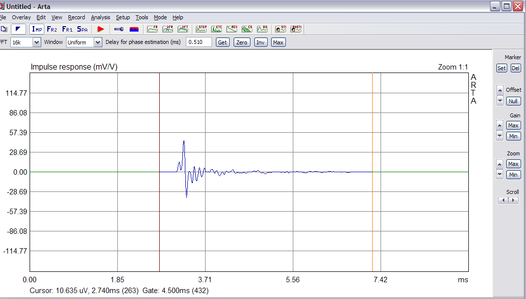
Теперь самое время рассказать более детально о главном недостатке одноканальных измерений – неопределенной опорной позиции курсора. С одной стороны никаких проблем – устанавливаем курсор перед импульсом, а маркер в максимум импульса и получаем задержку для расчета ФЧХ. Это так, но некорректная установка курсора резко проявляется на графике кумулятивного затухания спектра (Cumulative Spectral Decay). Вот как раз с помощью него мы и определим опорную позицию курсора. Насколько такой метод корректен, можно будет сделать вывод позже на основании результатов измерений двухканальным методом. Итак, смотрим на получившийся график импульсной характеристики (30).
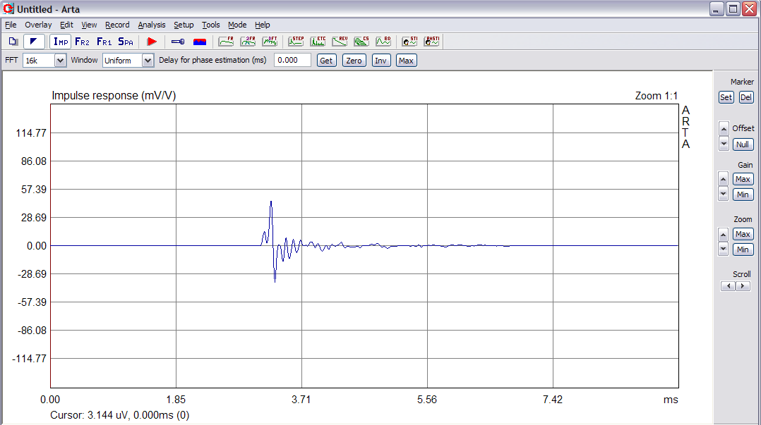
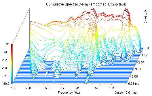
Сейчас курсор установлен в позицию 0 ms (0 samples), так и оставляем. Маркер устанавливаем сразу после импульса. В примере он стоит на отметке 4.646 ms. Чтобы избежать присутствия в сигнале ранних отражений, не устанавливайте маркер слишком далеко. Оптимальное временное окно – 4…5 ms. Нажимаем кнопку с буквами CS на панели инструментов или выбираем в меню Analysis – Cumulative spectrum. Откроется окно Cumulative Spectrum Setup (31). Этот график сокращенно называют CSD (Cumulative Spectral Decay).
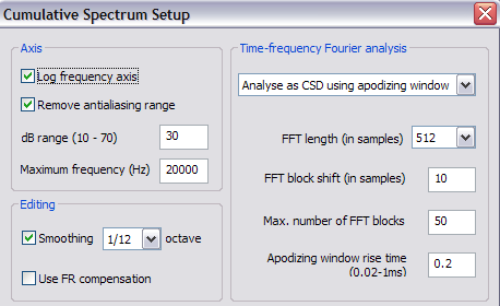
Галочка Log frequency axis отмечается, если требуется логарифмическая шкала частотного диапазона. Галочка Remove antialiasing range включает фильтрацию составляющих частотного диапазона в области Fs/2. dB range (10 – 70) и Maximum frequency (Hz) устанавливают соответственно отображаемый на экране динамический диапазон и верхнюю частоту. Поле Smoothing устанавливает сглаживание, а галочка Use FR compensation задействует компенсацию АЧХ, установленную в меню Setup – FR compensation (по понятным причинам я об этом меню не рассказывал). В правой части окна верхнее поле переключает тип анализа. При работе с импульсным откликом автоматически устанавливается тип Analyse as CSD using apodizing window. В поле FFT length (in samples) устанавливается количество сэмплов в блоке FFT. В случае если длина временного окна в сэмплах меньше FFT lenght/2, при запуске анализа программа выведет предупреждение. В поле FFT block shift (in samples) указывается длительность временной шкалы в сэмплах, а в поле Max. number of FFT blocks – количество блоков FFT, входящих во временную шкалу. В поле Apodizing window rise time (0.02-1 ms) указывается время открытия и закрытия окна анализа. Величина 0.2ms – это некоторый оптимум при анализе характеристик как в области низких, так и в области высоких частот. Производим установки и нажимаем OK.
Если наблюдается картина, подобная как на графике 32, необходимо увеличить временную шкалу (FFT block shift).
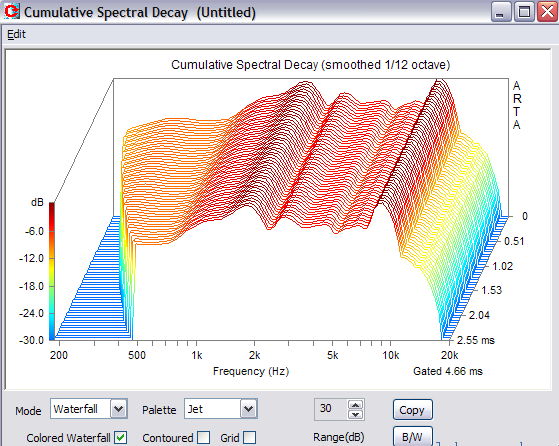
При использовании корректных настроек CSD, график должен выглядеть подобным образом (Fig 33).
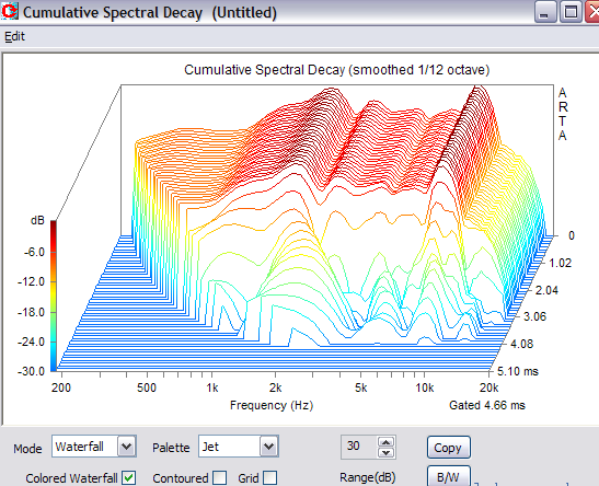
Из графика видно наличие блоков FFT с одинаковым содержимым. Это следствие некорректной установки курсора в окне импульсной характеристики – позиция курсора находится слишком рано по отношению к импульсу. Если же установить курсор в такую позицию, которая «отсечет» полезные данные, в окне CSD будет происходить анализ самих резонансных процессов, без сигнала их порождающего. Отразится это и на графике АЧХ. Поскольку на графике Waterfall не слишком удобно выражена временная шкала, предлагаю переключиться на сонограмму – в поле Mode выбираем Sonogram — 34.
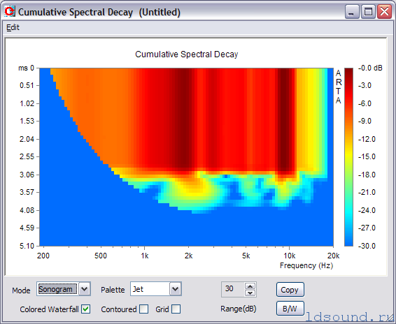
Здесь более наглядная временная шкала. Чтобы улучшить разрешение, отмечаем галочку Grid, а в настройках CSD станавим меньшую временную шкалу. Изменив настройки, выводим график — 35.

Видно, что спектр сигнала не содержит изменений до приблизительно 2.75 ms. Это и есть искомая позиция курсора. Закрываем окно. В окне импульсной характеристики устанавливаем курсор в позицию 2.75 ms (около этого значения), а маркер – в максимум импульса, получив тем самым значение задержки (36).
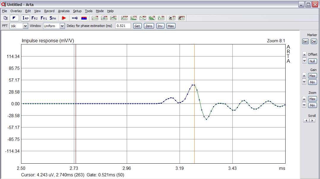
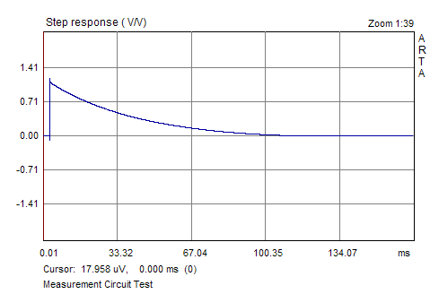
Здесь будет небольшое отступление по поводу максимума импульса. Как можно видеть выше, положение максимума импульса можно принять другим, если «развернуть» импульсную характеристику на 180 градусов. В таком случае максимум импульса окажется чуть дальше по времени. Это некорректная установка и она обязательно отразится на фазовой характеристике. Чтобы убедиться в том, что импульсная характеристика имеет «положительный» отклик, воспользуемся графиком переходной характеристики. Нажимаем на панели инструментов кнопку с надписью STEP, либо выбираем в меню Analysis – Step response. Откроется окно Step response (37).
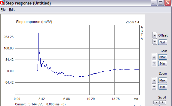
Можно видеть, переходная характеристика имеет «положительный» фронт. Если же переходная характеристика имеет «отрицательный» фронт (38), то необходимо в окне импульсной характеристики изменить фазу импульсного отклика с помощью кнопки Inv, расположенной на панели инструментов (либо через меню Edit – Invert). Можно провести повторное измерение, изменив полярность подключения динамика, либо повторное измерение с установленной галочкой Invert phase of input channel в окне — Impulse response measurement.
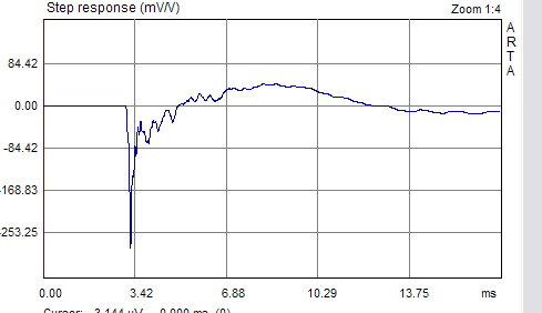
Вернемся к окну импульсной характеристики. Установили курсор, маркер и получили значение задержки. Теперь устанавливаем с помощью маркера окно измерений (Gate) около 4…5 ms (39).
Открываем окно CSD, производим установки и получаем результат (40).
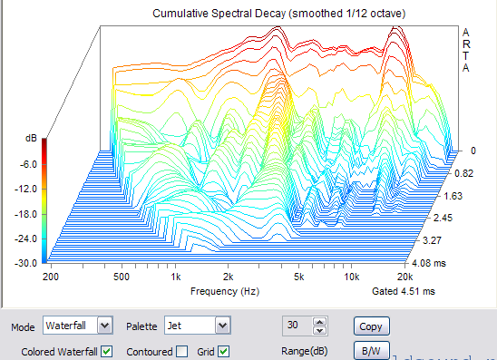
Убедиться в том, что график CSD отображается корректно, можно посмотрев график АЧХ (41).
Далее возвращаемся в окно импульсной характеристики. Установка курсора произведена, задержка рассчитана, теперь можно выбрать позицию маркера, определив тем самым окно измерений и нижнюю граничную частоту при анализе характеристик. Сейчас у меня произведено измерение в ближнем поле, поэтому я могу установить окно измерений длинным – около 50ms – и получить при анализе нижнюю граничную частоту 20Hz. Но когда производятся измерения в дальнем поле, либо помещение обладает неудовлетворительными акустическими свойствами, окно измерений желательно ограничивать еще до прихода первых отражений. Как их распознать в окне импульсной характеристики, показано на примере результата измерения ВЧ излучателя в дальнем поле (42).
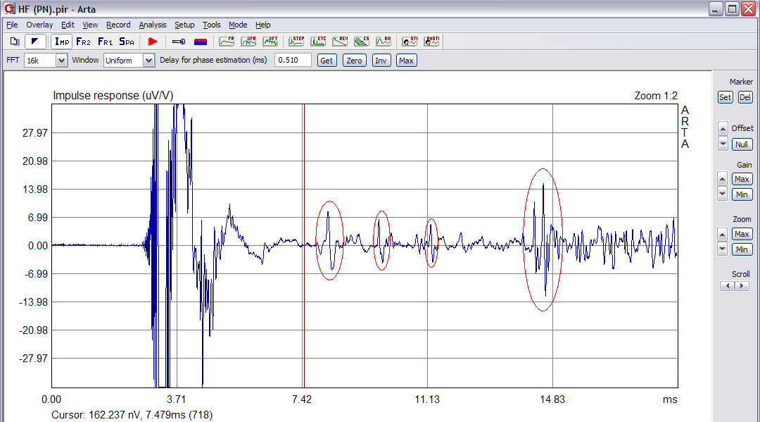
На изображении 42 курсор установлен в позицию, которая отображает границу чистого импульсного отклика. После курсора следуют отражения – ранние и поздние. Ранние отражения очень хорошо видны как повторяющийся три раза импульс. Поздние отражения имеют существенно большую амплитуду, в редких случаях даже сравнимую с амплитудой главного импульсного отклика.
Итак, определяем окно измерений. Для примера установили на 56.594 ms (5433 сэмпла). Теперь можно переходить к анализу результатов измерений и их экспорту в формат, поддерживаемый CAD-системами. Импульсную характеристику можно сохранить в формате Arta (*.pir), либо экспортировать в текстовый формат. Для анализа доступны следующие графики: АЧХ, ФЧХ, ГВЗ, ПХ, график зависимости энергии импульса от времени, кумулятивное затухание спектра и график распада. Для графиков АЧХ, ФЧХ и ГВЗ есть дополнительные меню, позволяющие просмотреть графики без сглаживания и меню с возможностью построения графиков с использованием двух временнЫх окон.
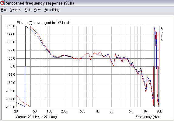
Кнопка с буквами FR, расположенная на панели инструментов, открывает меню Smoothed frequency response (через меню – Analysis – Single-gated smoothed Frequency response/Spectrum) – (43).
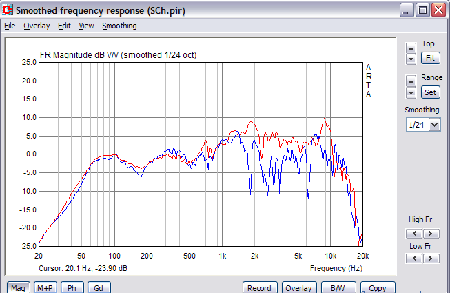
Внизу слева расположены кнопки Mag, M+P, Ph и Gd. С помощью них открываются графики соответственно АЧХ, АЧХ+ФЧХ, ФЧХ и ГВЗ. Справа в поле Smoothing из списка выбирается характеристика сглаживания. Щелчок правой кнопкой мыши на графике открывает экранное меню, где можно установить динамический и частотный диапазоны измерений. В меню File – Export… возможен экспорт результатов измерений в текстовый формат. Меню Overlay управляет слоями с кривыми. Можно «закрепить» на графике кривую для построения комбинированного графика. Например, для сравнения АЧХ на главной оси и с отклонением от оси (44).
С помощью пункта меню Edit – Scale level производится нормализация кривых (на приведенном выше графике кривые сначала нормализованы на частоте 100Hz и только потом совмещены). Меню LF box diffraction служит для компенсации так называемого «баффла». Фазовая характеристика может быть отображена как минимальная фаза (Minimum phase), избыточная фаза (Excess phase) или измеренная фаза (галочки с минимальной и избыточной фазы сняты). Активирование пункта Unwrap Phase отключает на графике ФЧХ «переворот» фазы при достижении значения -180 или 180 градусов. ГВЗ может быть рассчитано из избыточной фазы (пункт Excess group delay активирован) или из измеренной фазы (Excess group delay не отмечен).
Графики АЧХ, ФЧХ и ГВЗ возможно вывести с использованием комбинированного метода с двумя временнЫми окнами (Analysis – Dual-gated smoothed frequency response или кнопка с буквами 2FR на панели инструментов). Для этого в меню Setup – Analysis parameters (5) в полях Gate1 и Gate2 необходимо указать длительность каждого окна. В поле Gate1 возможна установка значений из диапазона 5…60 ms, а в поле Gate2 – 70…300ms.
Меню Analysis – Unsmoothed DFT frequency response/Spectrum или нажатие кнопки DFT на панели инструментов позволяет просмотреть графики АЧХ, ФЧХ и ГВЗ без сглаживания (45).
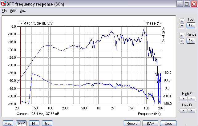
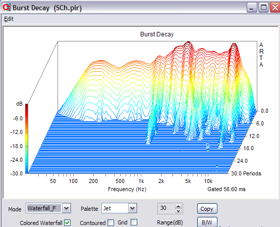
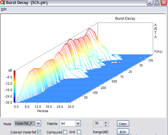
График распада (в меню Analysis – Burst decay или на панели инструментов кнопка BD) выглядит похожим на график CSD. Отличие их заключается в методе анализа. Разработчики Arta Software рекомендуют анализировать оба графика. В общем, по графику кумулятивного спектра хорошо видно наличие резонансов, но именно ярко выраженные резонансы нагляднее отображаются на графике Burst Decay (46 и 47).
Для оценки нелинейных искажений динамика, можно провести измерение зависимости уровня нелинейных искажений от частоты (меню Analysis – Frequency response and distortions). Для этого сначала переходим в меню Setup – Analysis parameters и в поле FFT length выбираем значение 131072. В окне Impulse response measurement переходим на вкладку Sweep. Если задействован двухканальный метод измерений, отключаем его и устанавливаем галочку Center peak of impulse response. В поле Sequence length выбираем значение 128k. Запускаем процесс измерений. Для примера, ниже (48) показан график нелинейных искажений широкополосного динамика 4А28 при подводимой мощности 1 Вт (3.46 v и нагрузке 12 Ом).
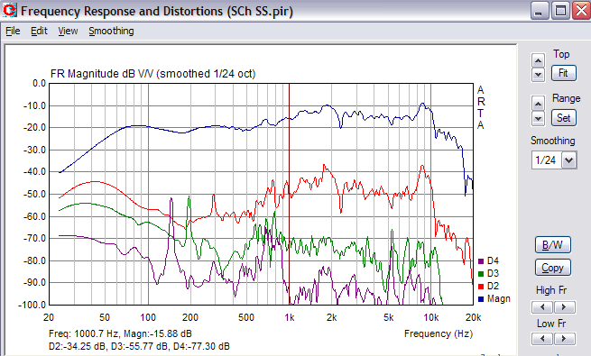
График отображает не суммарный уровень искажений, но отдельно гармоники. Если требуется знать THD, придется самостоятельно перевести децибелы в проценты и вычислить коэффициент гармоник. Проделав эту процедуру мы получим следующие результаты. THD на частоте 100 Hz составляет 1.535 %, на частоте 1 kHz – 1.937 %, на 10 kHz – 2.147 %.
Теперь о двухканальных измерениях. Производим подключение оборудования по схеме (28). В меню Setup – Calibrate devices (Figure 4) производим установку напряжения на выходе усилителя, а в меню Record – Impulse response/Signal time record (Figure 6) на вкладке Periodic Noise устанавливаем уровни входных сигналов в диапазоне -20….-10dB. При двухканальных измерениях Arta может самостоятельно определять задержку для расчета фазы. Я пользуюсь автоматическим расчетом только в том случае, если в окне импульсной характеристики невозможно определить положение максимума импульса. Это бывает, когда измеряется НЧ динамик с подключенным ФНЧ. Определение задержки производится в другом окне Arta – Dual channel – frequency response. Чтобы переключиться к нему, в меню Mode необходимо выбрать Dual channel – frequency response или на панели инструментов нажать кнопку Fr2. Окно Impulse response сменится (49).
Далее переходим в меню Setup – Measurement (50).
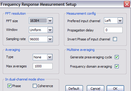
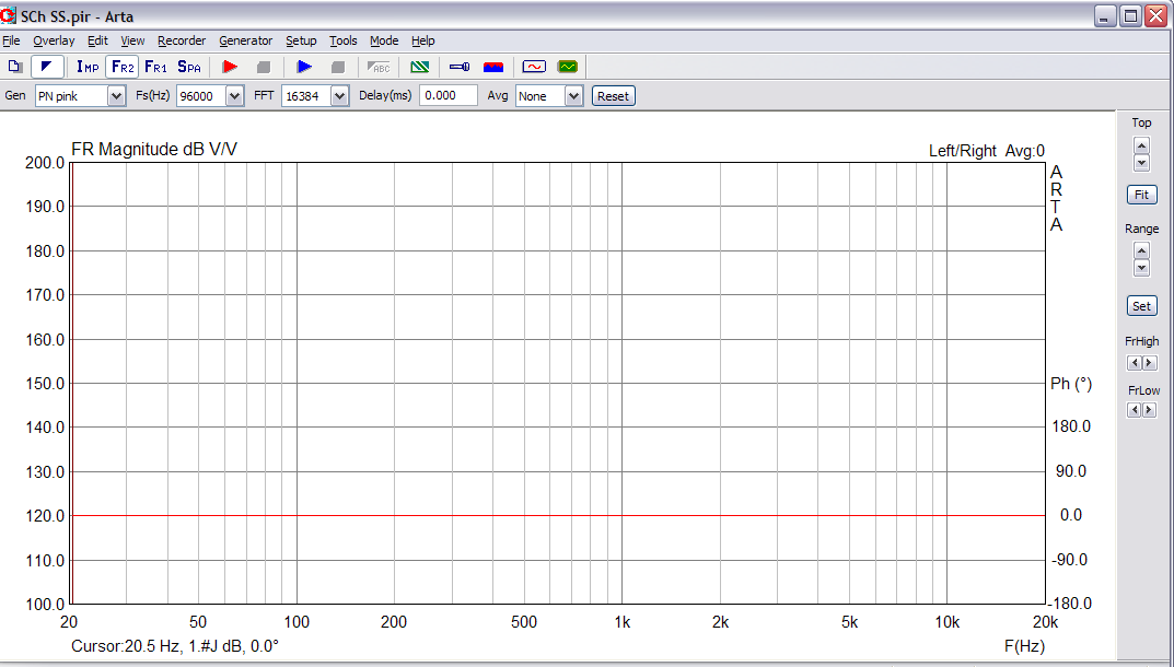
В поле FFT size указываем размер блока FFT – 16384, в поле Sampling rate – частоту дискретизации. Отмечаем галочку Phase, а в поле Prefered input channel выбираем канал, к которому подключен микрофон. В поле Propagation delay обязательно устанавливаем значение 0. На панели инструментов в поле Gen устанавливаем значение PN pink и проводим измерение (51).
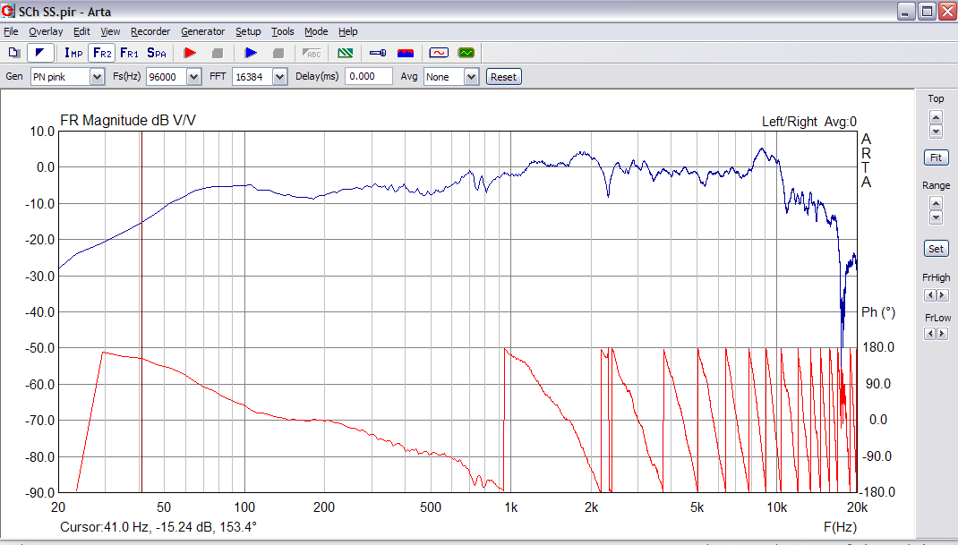
Фазовая характеристика, из-за отсутствия величины задержки, отображается с ошибкой. Автоматическое определение задержки производится через меню Record – Crosscorrelation/delay estimation (52).

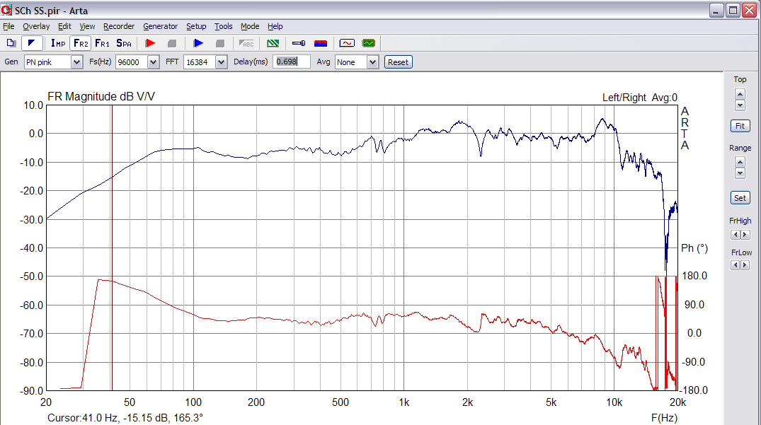
В поле Delay (ms) отображается значение задержки. Чтобы использовать это значение, достаточно нажать кнопку Accept. Происходит возврат в окно Fr2, где в поле Delay(ms) автоматически заносится значение задержки. Проводим измерение повторно (53).
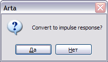
Теперь фазовая характеристика измерена корректно. Запоминаем в буфере обмена значение задержки, указанное в поле Delay(ms), и переходим в окно импульсной характеристики (кнопка Imp на панели инструментов или в меню Mode – Impulse response/Signal time record). При переключении программа предложит преобразовать результат измерений Fr2 в импульсную характеристику (54).
Можно согласиться, можно отказаться. Непринципиально, поскольку при конвертировании нарушается позиция, определенная как опорная для курсора при двухканальных измерениях. Поэтому измерение необходимо провести еще раз, но теперь уже через меню Record — Impulse response/Signal time record (Figure 6). Настраиваем поля для двухканального метода и проводим измерения. В окне импульсной характеристики опорная позиция курсора для двухканальных измерений определена точно — 300 сэмплов. Устанавливаем курсор в эту позицию, в поле Delay for phase estimation (ms) устанавливаем значение задержки, полученной при измерениях в Fr2. Осталось установить длину измерительного окна и можно приступать к анализу и экспорту (55).
Для сравнения, на графиках 56 и 57 представлены графики CSD при измерении соответственно одноканальным и двухканальным методами. На графике 58 синим цветом показана ФЧХ при измерении двухканальным методом, красным – при одноканальном методе. Разница явно небольшая.

Замечательная программа. Несущая в себе безграничные возможности для занятия всего вашего досуга.
Если вы нашли ошибку, пожалуйста, выделите фрагмент текста и нажмите Ctrl+Enter.
v1.2.3
Release info
This release includes binaries for macOS (10.13 — 12.0), Windows x64 (7, 8, 10, 11).
Desktop versions are available for download with a GPL3.0 license.
An iPadOS and iPhone version (commercial license) available here
New
- MLS+ noise
Improvements, Fixes and Optimisations
- Fixes

v1.2.2
Release info
This release includes binaries for macOS (10.13 — 12.0), Windows x64 (7, 8, 10, 11), Linux AppImage (build for Glibc 2.29 or above).
Desktop versions are available for download with a GPL3.0 license.
An iPadOS and iPhone version (commercial license) available here
New
- Apply mode for math source
- Peak and Crest Factor values in digital meters
- System time in digital indicators
- Pause for Level charts
- Common folder for all the files
Improvements, Fixes and Optimisations
- Option for inverse polarity for even channels in the generator
- Accurate tuning for weightings
- Many fixes
v1.2.1
Release info
This release includes binaries for macOS (10.13 — 12.0), Windows x64 (7, 8, 10, 11), Linux AppImage (build for Glibc 2.29 or above).
Desktop versions are available for download with a GPL3.0 license.
An iPadOS and iPhone version (commercial license) available here
New
- Added new Filter tool. You can generate source data to simulate Butterworth, Linkwitz Riley, and Bessel low pass or high pass filters.
Improvements, Fixes and Optimisations
- fix a few annoying bugs
- small UI optimisations

v1.2
Release info
This release includes binaries for macOS (10.13 — 12.0), Windows x64 (7, 8, 10, 11), Linux AppImage (build for Glibc 2.29 or above).
Desktop versions are available for download with a GPL3.0 license.
An iPadOS and iPhone version (commercial license) available here
New
-
Remote API
Remote API allows to share active and stored measurements data between different instances of Open Sound Meter. Also available for third party applications.
For example, you can use iPad as a wireless remote for your main measurement setup. -
Weightings
• Added: A, B and C weighting filters
• Added standard lines for weighting filters -
Quick calibration
94dB button in the measurement’s properties sets measurement channel gain correlated to SPL 94dBA slow. -
Level monitoring
For multichannel monitoring of current sound pressure levels (SPL) or digital levels (dBfs) Level chart added -
Digital meters
SPL and dBfs values could be observed as the digital meters -
Impedance
Impedance mode added for the magnitude measurements. You can calibrate interface for your sensor resistance in see results in Ohms. -
Burst noise
Improvements
-
Measurements
• Allow negative delay values
• Make impulse response time window equal to time frequency responses -
Generator
• Now it’s possible to select many outputs channels
• increase sweep period
• Rase maximum frequency in the generator up to 192kHz -
PPO
• Added 1 point per octave option
• Added PPO option for RTA line
• Added PPO off option for RTA bars -
Math Source
• Added ability to use math source as a source in other math source
• Added resulted impulse response to vectors functions -
Interface
• Add close button to popups
• Reset charts height by double click on the divider
• Step response extended limits
• Impulse response extended limits
• Enlarge popups for long titles (long channel names for example)
• Cmd + 4 (Ctrl+4) shortcut apply auto height for the charts
• Others small GUI improvements -
Audio
AudioSession (iOS) force set selected sample rate
Fixes
• Spectrogram reset ppo and binding loop
• Count for math source when cloned
• Spectrogram auto add sources
• Negative gain values in projects
• Others fixes
Optimisations
- Lots of CPU vector instructions optimisations
- Audio buffers allocation optimisations
v1.1
Release info
This release includes binaries for macOS (10.13 — 12.0), Windows x64 (7, 8, 10, 11), Linux AppImage (build for Glibc 2.29 or above).
Desktop versions are available for download with a GPL3.0 license.
An iPadOS version (commercial license) available here: https://apps.apple.com/app/id1552933259
New
-
Estimation delay
The estimation delay finder works in the background and can predict values up to 1.5 seconds at 48kHz. -
Recent files
The recent files menu allows you to quickly reopen any of the last sessions. -
Auto save
The application automatically saves the current project in the background. When next time you run the app, it will start from the last project. -
Reset button
Reset button added to the measurements properties. You can quickly reset average buffers. -
Loop
Internal loop buffer added, filled with generator samples. In each measurement, you can select loop buffer as a measurement or reference. -
CSV import
Any stored measurement could be exported in CSV format. -
Log impulse
Add log scale for y-axis on impulse response. -
Peak hold
Displaying peak value added to RTA chart and level meters. -
Import impulse
Now you can import impulse response data from CSV or WAV files. -
WAV export
Any stored measurement impulse could be exported in WAV format. -
SNR
A coherence chart has a new option to show data as SNR. -
Source selection
For each chart can be selected specific sources to show or hide. -
Ignore coherence
You can ignore coherence on the specific stored data and force it to be 100%.
Graphics
- Open GL2
On old computers, where Open GL3.3 is not available, the program will automatically fall back to Open GL2. That returns support of old video adapters on modern operating systems. Such as Intel HD3000 on Windows 10.
Math source
-
DB and power functions
Math source has now four options: vector, polar, dB and power. For the last three options, phase is calculated as polar type. -
Count
Added selection of sources counts: from 2 to 10. -
Coherence
The resulting coherence value is calculated as the weighted by module value sources average coherence. -
Polar phase
New math for polar type provides more useful results. -
Phase subtract
Phase subtract for polar types reworked. -
Auto name
If you didn’t change the name of the math source, it will be updating automatically with the selected type and function. -
Color labels
In the right tab, the source shows helping mini colour labels of selected sources.
Experimental function
-
Show experimental function
You can choose in the menu if you want to use or hide the experimental functions, that’s usually not needed but could be interesting in the labs or education. -
Crest factor
The crest factor chart shows the rate between peaks and average values measurements. -
Nyquist
Classic Nyquist plot is added. -
Phase delay
Added plot of phase delay.
Improvements
-
LTW
LTW transform prepares with knowledge of the current sample rate. That allows achieving the same frequencies list at different sample rates. -
Linear mode
A magnitude chart can show data not only as dB difference but linear too. -
FFT powers
Added 11 and 14 powers. -
Group delay
The charts renderer reworked. Now it shows smooth series with any PPO settings. -
Auto names
A new store has an auto name when created, it includes the name of the source and current time. -
Windows audio
Improvements of native Windows audio backend. Now it supports multichannel inputs. -
Support small screens
Layout can adapt for a tiny screen on microbooks or tablets -
Spectrogram level normalization
Levels now correspond to RTA values. -
Enable high dpi scaling
Support screens with high pixel density on all the platforms. Such as a 4K 13 inches monitor. -
Polarity button
The polarity reverse button clearly shows the status and took less space. -
Saved sources
Add saving and loading at the project file ELC and math source. -
Shift key
Use shift key for accuracy adjusting values. -
Last used folder
The application will remember the last folder you used to open a project. -
Scroll
Added scroll to the tablets side menu. -
Updater
When a new update is available, an updater will show you your current version and suggested one.
Fixes
-
Reset buffers
Fix for bug: sometimes buffers weren’t reset. -
Generator
Fix for the level ignoring bug when generators works with wav file. -
Metal renderer
Fix crash on resize chart. -
Import bad files
If an imported file has invalid values, «*» instead of digits, this value won’t be ignored and imported as zero. -
Load bad files
Fix crash on load disabled measurement. -
Audio
Fixes for audio client for Windows 7. -
Layout
Fixes lots of layout issues -
Other
Lots of major and minor fixes
Notes
- Optimization
Added a lot of optimizations for better CPU and GPU loads.
v1.0.5
Release info
This release includes binaries for macOS (10.13 — 11.1), Windows x64 (7, 8, 10)
Desktop versions are available for download with a GPL3.0 license.
An iPadOS version (commercial license) available here: https://apps.apple.com/app/id1552933259
New
- Target trace
Use Cmd+T (Ctrl+T) shortcut to see target trace on magnitude response.
Fixes
- OpenGL render for NVidia drivers Windows 10
- small UI fixes
v1.0.1
Release info
Fixes for v1.0 release
This release includes binaries for macOS (10.13 — 11.1), Windows x64 (7, 8, 10), Linux AppImage (build for Glibc 2.29 or above).
Desktop versions are available for download with a GPL3.0 license.
An iPadOS version (commercial license) available here: https://apps.apple.com/app/id1552933259
Improvements
-
Mouse wheel
The mouse wheel can be used for charts scroll. -
Show positive phase values option
For phase chart added an option to select how should be phase show: from -180 to 180 or from 0 to 360.
Fixes
- OpenGL render for Windows 10
- Font render for macOS
- auto dark mode for macOS
v1.0
Release info
This release includes binaries for macOS (10.13 — 11.1), Windows x64 (7, 8, 10), Linux AppImage (build for Glibc 2.29 or above).
Desktop versions are available for download with a GPL3.0 license.
An iPadOS version (commercial license) available here: https://apps.apple.com/app/id1552933259
New
-
Audio device connection
Full new module for audio interfaces: -
AudioSessions (iOS)
-
CoreAudio (macOS)
-
WASPAPI (Windows)
-
ASIO (Windows)
-
ALSA (Linux)
-
OpenGL3.3 render engine
Full new rendering module. Improved speed and GPU usage. -
Apple Metal render engine
iOS uses Apple metal rendering. -
Multitouch control
Scroll and scale charts with multitouch gestures on touchscreen or touchpad. The phase chart can be infinitely rotated. -
M-Noise™ test signal
This signal can be used only if the selected audio interface works at 96kHz. -
Reset chart
Chart’s X and Y ranges can be reset by double click. -
Cursor lines
Thin helper lines moved with a cursor and show the current position on all the charts. -
Text selection
At all text inputs, text can be selected by mouse. At the spinboxes text automatically selected when clicked. -
Offline tune
Stored data can be adjusted by the gain, time and polarity. Also, it has a magnitude inverse option. -
Source clone
Sources can be quick cloned
Mathematic
-
Fourier transform normalization
RTA chart will show the same level whatever power of FT selected -
Group delay
Rewritten math for group delay chart. -
Step response
More stable result. Added a selectable zero point.
Improvements
-
Auto dark mode
dark mode follows systems appearance -
Coherence threshold line added
The coherence chart now has a customizable target line -
Cursor values
Position of cursor values changed according to position on the chart. It Will never goes out of bounds. -
Estimated delay
The button shows the proposed value (was E). Tooltip shows the delta between current and proposed. -
Ask before close
Prevents accidentally closing the program. -
Line colors
Charts lines became less contrast. -
Generator
- Level for the generator can be adjusted in the right bar.
- Added none option for the output
-
Calculator
Expanded ranges of the values. -
Video adapter
Show error if the adapter doesn’t support OpenGL3.3
Fixes
- auto select correct video adapter on MacBook Pro with two adapters
- ELC freeze on Windows platform
- Charts spline function fixed
- Title for the chart source filter
- and other minor fixes
Notes
M‑Noise is a trademark of Meyer Sound Laboratories. https://m-noise.org/
v0.3.1
Release info
This release includes binaries for macOS (10.13 — 11.1), Windows x64 (7, 8, 10), Linux (Ubuntu 19.10 AppImage)
New
-
Donations
New service for donation and new About window -
CSV data Import
Improvements
-
Spectrogram
Added properties for defining level (in dB) for blue, green and red colours -
Math source
Added selector for vector or polar operation -
Stored
To the auto-notes added: gain, selected device and its channels
Fixes
- for MOTU and RME drivers
- calibration files
Notes
- Linux
AppImage is built with Ubuntu 19.10. If this AppImage is not working for you, you can build the application with Qt5.15.2 yourself.
v0.3
Release info
This release includes binaries for macOS (10.13, 10.14, 10.15), Windows x64 (7, 8, 10), Linux (Ubuntu 19.10 AppImage)
New
-
Log time windows transform
in LTW transform frequencies have logarithmic step size. Each frequency has its own time window (drop with frequency rise)

-
Step response chart

-
Equal loudness contours
-
Import and export in txt format
-
Gain adjustment for the measurement
Improvements
-
Charts
Z-order of the series corresponds to the order of the sources. The selected source is always on top and has a bold line. -
Sweep generator
Settings for the duration of the sweep added
Fixes
- Issues fixed
- Improved stability
- FRD file format export
Notes
- Linux
AppImage is built with Ubuntu 19.10. If this AppImage is not working for you, you can build the application with Qt5.15.2 yourself.
-
#1
Learned about this today. Seems similar to some of the more expensive measurement programs (smaart, systune) with real time measurements via a loop back reference for Phase, Coherence, Magnitude, etc. Right now this is freeware much like REW.
https://opensoundmeter.com/
v1.2.2
Release info
This release includes binaries for macOS (10.13 — 12.0), Windows x64 (7, 8, 10, 11), Linux AppImage (build for Glibc 2.29 or above).
Desktop versions are available for download with a GPL3.0 license.
An iPadOS and iPhone version (commercial license) available here
New
- Apply mode for math source
- Peak and Crest Factor values in digital meters
- System time in digital indicators
- Pause for Level charts
- Common folder for all the files
Improvements, Fixes and Optimisations
- Option for inverse polarity for even channels in the generator
- Accurate tuning for weightings
- Many fixes
v1.2.1
Release info
This release includes binaries for macOS (10.13 — 12.0), Windows x64 (7, 8, 10, 11), Linux AppImage (build for Glibc 2.29 or above).
Desktop versions are available for download with a GPL3.0 license.
An iPadOS and iPhone version (commercial license) available here
New
- Added new Filter tool. You can generate source data to simulate Butterworth, Linkwitz Riley, and Bessel low pass or high pass filters.
Improvements, Fixes and Optimisations
- fix a few annoying bugs
- small UI optimisations
v1.2
Release info
This release includes binaries for macOS (10.13 — 12.0), Windows x64 (7, 8, 10, 11), Linux AppImage (build for Glibc 2.29 or above).
Desktop versions are available for download with a GPL3.0 license.
An iPadOS and iPhone version (commercial license) available here
New
-
Remote API
Remote API allows to share active and stored measurements data between different instances of Open Sound Meter. Also available for third party applications.
For example, you can use iPad as a wireless remote for your main measurement setup. -
Weightings
• Added: A, B and C weighting filters
• Added standard lines for weighting filters -
Quick calibration
94dB button in the measurement’s properties sets measurement channel gain correlated to SPL 94dBA slow. -
Level monitoring
For multichannel monitoring of current sound pressure levels (SPL) or digital levels (dBfs) Level chart added -
Digital meters
SPL and dBfs values could be observed as the digital meters -
Impedance
Impedance mode added for the magnitude measurements. You can calibrate interface for your sensor resistance in see results in Ohms. -
Burst noise
Improvements
-
Measurements
• Allow negative delay values
• Make impulse response time window equal to time frequency responses -
Generator
• Now it’s possible to select many outputs channels
• increase sweep period
• Rase maximum frequency in the generator up to 192kHz -
PPO
• Added 1 point per octave option
• Added PPO option for RTA line
• Added PPO off option for RTA bars -
Math Source
• Added ability to use math source as a source in other math source
• Added resulted impulse response to vectors functions -
Interface
• Add close button to popups
• Reset charts height by double click on the divider
• Step response extended limits
• Impulse response extended limits
• Enlarge popups for long titles (long channel names for example)
• Cmd + 4 (Ctrl+4) shortcut apply auto height for the charts
• Others small GUI improvements -
Audio
AudioSession (iOS) force set selected sample rate
Fixes
• Spectrogram reset ppo and binding loop
• Count for math source when cloned
• Spectrogram auto add sources
• Negative gain values in projects
• Others fixes
Optimisations
- Lots of CPU vector instructions optimisations
- Audio buffers allocation optimisations
v1.1
Release info
This release includes binaries for macOS (10.13 — 12.0), Windows x64 (7, 8, 10, 11), Linux AppImage (build for Glibc 2.29 or above).
Desktop versions are available for download with a GPL3.0 license.
An iPadOS version (commercial license) available here: https://apps.apple.com/app/id1552933259
New
-
Estimation delay
The estimation delay finder works in the background and can predict values up to 1.5 seconds at 48kHz. -
Recent files
The recent files menu allows you to quickly reopen any of the last sessions. -
Auto save
The application automatically saves the current project in the background. When next time you run the app, it will start from the last project. -
Reset button
Reset button added to the measurements properties. You can quickly reset average buffers. -
Loop
Internal loop buffer added, filled with generator samples. In each measurement, you can select loop buffer as a measurement or reference. -
CSV import
Any stored measurement could be exported in CSV format. -
Log impulse
Add log scale for y-axis on impulse response. -
Peak hold
Displaying peak value added to RTA chart and level meters. -
Import impulse
Now you can import impulse response data from CSV or WAV files. -
WAV export
Any stored measurement impulse could be exported in WAV format. -
SNR
A coherence chart has a new option to show data as SNR. -
Source selection
For each chart can be selected specific sources to show or hide. -
Ignore coherence
You can ignore coherence on the specific stored data and force it to be 100%.
Graphics
- Open GL2
On old computers, where Open GL3.3 is not available, the program will automatically fall back to Open GL2. That returns support of old video adapters on modern operating systems. Such as Intel HD3000 on Windows 10.
Math source
-
DB and power functions
Math source has now four options: vector, polar, dB and power. For the last three options, phase is calculated as polar type. -
Count
Added selection of sources counts: from 2 to 10. -
Coherence
The resulting coherence value is calculated as the weighted by module value sources average coherence. -
Polar phase
New math for polar type provides more useful results. -
Phase subtract
Phase subtract for polar types reworked. -
Auto name
If you didn’t change the name of the math source, it will be updating automatically with the selected type and function. -
Color labels
In the right tab, the source shows helping mini colour labels of selected sources.
Experimental function
-
Show experimental function
You can choose in the menu if you want to use or hide the experimental functions, that’s usually not needed but could be interesting in the labs or education. -
Crest factor
The crest factor chart shows the rate between peaks and average values measurements. -
Nyquist
Classic Nyquist plot is added. -
Phase delay
Added plot of phase delay.
Improvements
-
LTW
LTW transform prepares with knowledge of the current sample rate. That allows achieving the same frequencies list at different sample rates. -
Linear mode
A magnitude chart can show data not only as dB difference but linear too. -
FFT powers
Added 11 and 14 powers. -
Group delay
The charts renderer reworked. Now it shows smooth series with any PPO settings. -
Auto names
A new store has an auto name when created, it includes the name of the source and current time. -
Windows audio
Improvements of native Windows audio backend. Now it supports multichannel inputs. -
Support small screens
Layout can adapt for a tiny screen on microbooks or tablets -
Spectrogram level normalization
Levels now correspond to RTA values. -
Enable high dpi scaling
Support screens with high pixel density on all the platforms. Such as a 4K 13 inches monitor. -
Polarity button
The polarity reverse button clearly shows the status and took less space. -
Saved sources
Add saving and loading at the project file ELC and math source. -
Shift key
Use shift key for accuracy adjusting values. -
Last used folder
The application will remember the last folder you used to open a project. -
Scroll
Added scroll to the tablets side menu. -
Updater
When a new update is available, an updater will show you your current version and suggested one.
Fixes
-
Reset buffers
Fix for bug: sometimes buffers weren’t reset. -
Generator
Fix for the level ignoring bug when generators works with wav file. -
Metal renderer
Fix crash on resize chart. -
Import bad files
If an imported file has invalid values, «*» instead of digits, this value won’t be ignored and imported as zero. -
Load bad files
Fix crash on load disabled measurement. -
Audio
Fixes for audio client for Windows 7. -
Layout
Fixes lots of layout issues -
Other
Lots of major and minor fixes
Notes
- Optimization
Added a lot of optimizations for better CPU and GPU loads.
v1.0.5
Release info
This release includes binaries for macOS (10.13 — 11.1), Windows x64 (7, 8, 10)
Desktop versions are available for download with a GPL3.0 license.
An iPadOS version (commercial license) available here: https://apps.apple.com/app/id1552933259
New
- Target trace
Use Cmd+T (Ctrl+T) shortcut to see target trace on magnitude response.
Fixes
- OpenGL render for NVidia drivers Windows 10
- small UI fixes
v1.0.1
Release info
Fixes for v1.0 release
This release includes binaries for macOS (10.13 — 11.1), Windows x64 (7, 8, 10), Linux AppImage (build for Glibc 2.29 or above).
Desktop versions are available for download with a GPL3.0 license.
An iPadOS version (commercial license) available here: https://apps.apple.com/app/id1552933259
Improvements
-
Mouse wheel
The mouse wheel can be used for charts scroll. -
Show positive phase values option
For phase chart added an option to select how should be phase show: from -180 to 180 or from 0 to 360.
Fixes
- OpenGL render for Windows 10
- Font render for macOS
- auto dark mode for macOS
v1.0
Release info
This release includes binaries for macOS (10.13 — 11.1), Windows x64 (7, 8, 10), Linux AppImage (build for Glibc 2.29 or above).
Desktop versions are available for download with a GPL3.0 license.
An iPadOS version (commercial license) available here: https://apps.apple.com/app/id1552933259
New
-
Audio device connection
Full new module for audio interfaces: -
AudioSessions (iOS)
-
CoreAudio (macOS)
-
WASPAPI (Windows)
-
ASIO (Windows)
-
ALSA (Linux)
-
OpenGL3.3 render engine
Full new rendering module. Improved speed and GPU usage. -
Apple Metal render engine
iOS uses Apple metal rendering. -
Multitouch control
Scroll and scale charts with multitouch gestures on touchscreen or touchpad. The phase chart can be infinitely rotated. -
M-Noise™ test signal
This signal can be used only if the selected audio interface works at 96kHz. -
Reset chart
Chart’s X and Y ranges can be reset by double click. -
Cursor lines
Thin helper lines moved with a cursor and show the current position on all the charts. -
Text selection
At all text inputs, text can be selected by mouse. At the spinboxes text automatically selected when clicked. -
Offline tune
Stored data can be adjusted by the gain, time and polarity. Also, it has a magnitude inverse option. -
Source clone
Sources can be quick cloned
Mathematic
-
Fourier transform normalization
RTA chart will show the same level whatever power of FT selected -
Group delay
Rewritten math for group delay chart. -
Step response
More stable result. Added a selectable zero point.
Improvements
-
Auto dark mode
dark mode follows systems appearance -
Coherence threshold line added
The coherence chart now has a customizable target line -
Cursor values
Position of cursor values changed according to position on the chart. It Will never goes out of bounds. -
Estimated delay
The button shows the proposed value (was E). Tooltip shows the delta between current and proposed. -
Ask before close
Prevents accidentally closing the program. -
Line colors
Charts lines became less contrast. -
Generator
- Level for the generator can be adjusted in the right bar.
- Added none option for the output
-
Calculator
Expanded ranges of the values. -
Video adapter
Show error if the adapter doesn’t support OpenGL3.3
Fixes
- auto select correct video adapter on MacBook Pro with two adapters
- ELC freeze on Windows platform
- Charts spline function fixed
- Title for the chart source filter
- and other minor fixes
Notes
M‑Noise is a trademark of Meyer Sound Laboratories. https://m-noise.org/
v0.3.1
Release info
This release includes binaries for macOS (10.13 — 11.1), Windows x64 (7, 8, 10), Linux (Ubuntu 19.10 AppImage)
New
-
Donations
New service for donation and new About window -
CSV data Import
Improvements
-
Spectrogram
Added properties for defining level (in dB) for blue, green and red colours -
Math source
Added selector for vector or polar operation -
Stored
To the auto-notes added: gain, selected device and its channels
Fixes
- for MOTU and RME drivers
- calibration files
Notes
- Linux
AppImage is built with Ubuntu 19.10. If this AppImage is not working for you, you can build the application with Qt5.15.2 yourself.
v0.3
Release info
This release includes binaries for macOS (10.13, 10.14, 10.15), Windows x64 (7, 8, 10), Linux (Ubuntu 19.10 AppImage)
New
-
Log time windows transform
in LTW transform frequencies have logarithmic step size. Each frequency has its own time window (drop with frequency rise)
-
Step response chart
-
Equal loudness contours
-
Import and export in txt format
-
Gain adjustment for the measurement
Improvements
-
Charts
Z-order of the series corresponds to the order of the sources. The selected source is always on top and has a bold line. -
Sweep generator
Settings for the duration of the sweep added
Fixes
- Issues fixed
- Improved stability
- FRD file format export
Notes
- Linux
AppImage is built with Ubuntu 19.10. If this AppImage is not working for you, you can build the application with Qt5.15.2 yourself.
-
#1
Learned about this today. Seems similar to some of the more expensive measurement programs (smaart, systune) with real time measurements via a loop back reference for Phase, Coherence, Magnitude, etc. Right now this is freeware much like REW.
https://opensoundmeter.com/
-
Thread Starter
-
#2
Played with this today and compared it to a stand alone Motu m4 and dayton emm-6 to a usb Dayton Umm-6 and a cheap $15 usb sound card with a headphone splitter. Seems to be pretty decent results. Definitely some clock drift issues above like 8k with the usb loopback, so using above that may get difficult.
To use the usb sound card device and usb microphone you’ll need to have the ability to make an aggregate device. In mac open audio midi and add a new device. For windows use Asio4All. Google those directions if you want to know how more.
This is what I am using:
Single I/O device setup:
Motu M4
Dayton Emm-6 microphone
USB devices:
Dayton Umm-6 microphone
External USB sound card
Headphone Splitter
Setup:
Note: These are without any microphone calibration files.
Smaart Results
Open Sound Meter: Was actually really easy to use, probably took less time to setup compared to Smaart.
Moral of this story…For $15 and open sound meter, you can get some decent results, especially below 8k. Above 8k, and you have clock drift issues. You could see the results kept changing every time the clock was adjusted. So if you want to use it above that, you’ll need to invest more money.
*Edited on 2/8/21 Open sound meter picture to not have smoothing.*
Last edited:
-
Thread Starter
-
#3
Here are some final thoughts after playing some more with Open Sound Meter vs. Smaart. I have been playing with smaart only for a little bit (The demo then I purchased my own copy recently).
Initial measurement setup -> Open Sound Meter was easier
Changing setups -> Smaart is easier
Setting up and Measuring again -> Smaart is easier (it remembers and you can easily create pairs to switch)
Saving -> Smaart auto saves everything and recalls everything upon opening, Open sound meter doesn’t even warn you before you exit….ask me how I know.
Overall Open sound meter works well enough if you are just tuning one thing and then putting everything away. It will take overall more time because you have to change all of the settings every time you open it. It doesn’t remember if you unplug something. It does seem to remember if everything is ALWAYS plugged in. Like close it on accident and re-open without changing anything it will remember. Smaart just remembers all of your stuff everytime. I created a m4 and a usb sound card setting and switch between the two instantly when I was taking those measurements. Smaart always remembers your settings, probably that autosave everything.
Smaart has a lot of keyboard shortcuts that makes things super quick to measure.
So overall, I can definitely recommend open sound meter and if you aren’t using it (even with a usb microphone and a cheap loopback device) you are missing out on very valuable information.
If you are going to be measuring a lot of different things, I would at least get a XLR microphone and something like a motu m2 or focusrite 2i2 and use open sound meter. I would even suggest purchasing Smaart di 2, it will save you a bunch of time. I will be using it when I teach waves to my physics classes and my wife is also a theatre teacher so will be showing her how to use it and her tech students for their shows. Smaart was worth the purchase for me for that stuff.
If you are just starting out in tuning, invest in a XLR measurment microphone like the dayton Emm6 and a device to interface with your computer. It might cost a little more upfront but so worth it compared to a usb microphone since you can use open sound meter with that and get useable results all the way up to 20 khz.
Dayton Emm-6
Focusrite 2i2 3rd gen refurb
Focusrite 2i2 2nd gen
Motu M2
Motu M4
A combination of the Dayton Mic and one of those interfaces would range anywhere from about $160-$300.
If you already have a XLR mic and interface. Give the Open Sound Meter a try and post your results here!
Last edited:
-
#4
A little addition.
Noted «clock drift» issue was an issue of the aggregated device, but not a software bug.
This image shows a difference between internal vs external loop when the aggregated device was build right. Both measurements are very close and stable.
-
Thread Starter
-
#5
Yes, it was definitely a device clock drift issue not a software issue. Even smaart had the same issue, so 100% the setup and the stuff I was using for that setup.
I was trying this because almost everyone these days buys a usb microphone like the Dayton or minidsp. I was seeing if it would work, overall it is still a yes! I’m gonna try soundflower this weekend and see if it works better (Pavel used it for his demo above)
To clear up any confusion this is what I did on the second setup, things weren’t exactly placed like that but it helps illustrate the point.
This was the aggregate device
Last edited:
-
Thread Starter
-
#6
This was the first setup with the motu
-
Thread Starter
-
#7
Also, I am pretty sure psmokotnin is the creator of Open Sound Meter. It is so awesome to have people like this that are willing to help on their stuff in a forum!

-
#9
For Russian speakers, an interview on OSM:
-
Thread Starter
-
#10
Now time to find someone to translate that for me
-
#11
Now time to find someone to translate that for me
")
I can listen to it at some point and quote a few interesting things.
-
Thread Starter
-
#12
I know @joentell is now using this program, anyone else try it out yet? Post your thoughts/results after using it!
It really is a game changer to be able to measure phase in real time! You can do fun things with this to get it to align the best possible.
I was eq’ing some speakers I built (the pe cnotes that are in my picture) and a sub.
This was the best I could get at first:
Note: These are Smaart pictures but open sound meter does the same thing.
You can see in the middle the real time phase. The orange is the sub, the green and pink are each speaker individually and the blue is both speakers. Everything was lined up the best I could get it by just introducing time delays. This is what I would normally just do in REW and get it the best possible after HOURS of work in sweeps and small adjustments. This was after spending countless hours trying to figure out how to get REW to properly measure phase that was useable. It is not the easiest process.
I would have never thought of doing this if I hadn’t seen the phase in real time. The picture below, I flipped the polarity of the sub because this aligned the slope of the phase better, and then used time delay to get them to line up. The next step would be all pass filters, but this wasn’t needed after doing the polarity flip. You can see, the sub phase, left speaker phase, and right speaker phase are all locked on to each other VERY well.
This is how you properly integrate subs with mains.
This also took me like an hour or so to learn to use the program and about an hours worth of time to do this. In REW, this would have been at minimum a few hours probably over the course of a few days to get not even close to this. There is no more guesswork here. This is about the best it is ever going to get.
Last edited:
-
Thread Starter
-
#13
-
Thread Starter
-
#14
-
Thread Starter
-
#15
-
Thread Starter
-
#16
@psmokotnin
Any way to do EQ on screen? Like REW EQ window does? Would be cool to be able to apply eq with inverted magnitude to either the RTA or magnitude screen. That way Q, gain, frequency is done.
I know some have tricked their systems with measuring the output of their dsp and being able to do that, but that is harder than just having it built in.
Example Like this, but would be very cool to not have to measure the dsp output and just be able to do this:
v1.2.3
Release info
This release includes binaries for macOS (10.13 — 12.0), Windows x64 (7, 8, 10, 11).
Desktop versions are available for download with a GPL3.0 license.
An iPadOS and iPhone version (commercial license) available here
New
- MLS+ noise
Improvements, Fixes and Optimisations
- Fixes
v1.2.2
Release info
This release includes binaries for macOS (10.13 — 12.0), Windows x64 (7, 8, 10, 11), Linux AppImage (build for Glibc 2.29 or above).
Desktop versions are available for download with a GPL3.0 license.
An iPadOS and iPhone version (commercial license) available here
New
- Apply mode for math source
- Peak and Crest Factor values in digital meters
- System time in digital indicators
- Pause for Level charts
- Common folder for all the files
Improvements, Fixes and Optimisations
- Option for inverse polarity for even channels in the generator
- Accurate tuning for weightings
- Many fixes
v1.2.1
Release info
This release includes binaries for macOS (10.13 — 12.0), Windows x64 (7, 8, 10, 11), Linux AppImage (build for Glibc 2.29 or above).
Desktop versions are available for download with a GPL3.0 license.
An iPadOS and iPhone version (commercial license) available here
New
- Added new Filter tool. You can generate source data to simulate Butterworth, Linkwitz Riley, and Bessel low pass or high pass filters.
Improvements, Fixes and Optimisations
- fix a few annoying bugs
- small UI optimisations
v1.2
Release info
This release includes binaries for macOS (10.13 — 12.0), Windows x64 (7, 8, 10, 11), Linux AppImage (build for Glibc 2.29 or above).
Desktop versions are available for download with a GPL3.0 license.
An iPadOS and iPhone version (commercial license) available here
New
-
Remote API
Remote API allows to share active and stored measurements data between different instances of Open Sound Meter. Also available for third party applications.
For example, you can use iPad as a wireless remote for your main measurement setup. -
Weightings
• Added: A, B and C weighting filters
• Added standard lines for weighting filters -
Quick calibration
94dB button in the measurement’s properties sets measurement channel gain correlated to SPL 94dBA slow. -
Level monitoring
For multichannel monitoring of current sound pressure levels (SPL) or digital levels (dBfs) Level chart added -
Digital meters
SPL and dBfs values could be observed as the digital meters -
Impedance
Impedance mode added for the magnitude measurements. You can calibrate interface for your sensor resistance in see results in Ohms. -
Burst noise
Improvements
-
Measurements
• Allow negative delay values
• Make impulse response time window equal to time frequency responses -
Generator
• Now it’s possible to select many outputs channels
• increase sweep period
• Rase maximum frequency in the generator up to 192kHz -
PPO
• Added 1 point per octave option
• Added PPO option for RTA line
• Added PPO off option for RTA bars -
Math Source
• Added ability to use math source as a source in other math source
• Added resulted impulse response to vectors functions -
Interface
• Add close button to popups
• Reset charts height by double click on the divider
• Step response extended limits
• Impulse response extended limits
• Enlarge popups for long titles (long channel names for example)
• Cmd + 4 (Ctrl+4) shortcut apply auto height for the charts
• Others small GUI improvements -
Audio
AudioSession (iOS) force set selected sample rate
Fixes
• Spectrogram reset ppo and binding loop
• Count for math source when cloned
• Spectrogram auto add sources
• Negative gain values in projects
• Others fixes
Optimisations
- Lots of CPU vector instructions optimisations
- Audio buffers allocation optimisations
v1.1
Release info
This release includes binaries for macOS (10.13 — 12.0), Windows x64 (7, 8, 10, 11), Linux AppImage (build for Glibc 2.29 or above).
Desktop versions are available for download with a GPL3.0 license.
An iPadOS version (commercial license) available here: https://apps.apple.com/app/id1552933259
New
-
Estimation delay
The estimation delay finder works in the background and can predict values up to 1.5 seconds at 48kHz. -
Recent files
The recent files menu allows you to quickly reopen any of the last sessions. -
Auto save
The application automatically saves the current project in the background. When next time you run the app, it will start from the last project. -
Reset button
Reset button added to the measurements properties. You can quickly reset average buffers. -
Loop
Internal loop buffer added, filled with generator samples. In each measurement, you can select loop buffer as a measurement or reference. -
CSV import
Any stored measurement could be exported in CSV format. -
Log impulse
Add log scale for y-axis on impulse response. -
Peak hold
Displaying peak value added to RTA chart and level meters. -
Import impulse
Now you can import impulse response data from CSV or WAV files. -
WAV export
Any stored measurement impulse could be exported in WAV format. -
SNR
A coherence chart has a new option to show data as SNR. -
Source selection
For each chart can be selected specific sources to show or hide. -
Ignore coherence
You can ignore coherence on the specific stored data and force it to be 100%.
Graphics
- Open GL2
On old computers, where Open GL3.3 is not available, the program will automatically fall back to Open GL2. That returns support of old video adapters on modern operating systems. Such as Intel HD3000 on Windows 10.
Math source
-
DB and power functions
Math source has now four options: vector, polar, dB and power. For the last three options, phase is calculated as polar type. -
Count
Added selection of sources counts: from 2 to 10. -
Coherence
The resulting coherence value is calculated as the weighted by module value sources average coherence. -
Polar phase
New math for polar type provides more useful results. -
Phase subtract
Phase subtract for polar types reworked. -
Auto name
If you didn’t change the name of the math source, it will be updating automatically with the selected type and function. -
Color labels
In the right tab, the source shows helping mini colour labels of selected sources.
Experimental function
-
Show experimental function
You can choose in the menu if you want to use or hide the experimental functions, that’s usually not needed but could be interesting in the labs or education. -
Crest factor
The crest factor chart shows the rate between peaks and average values measurements. -
Nyquist
Classic Nyquist plot is added. -
Phase delay
Added plot of phase delay.
Improvements
-
LTW
LTW transform prepares with knowledge of the current sample rate. That allows achieving the same frequencies list at different sample rates. -
Linear mode
A magnitude chart can show data not only as dB difference but linear too. -
FFT powers
Added 11 and 14 powers. -
Group delay
The charts renderer reworked. Now it shows smooth series with any PPO settings. -
Auto names
A new store has an auto name when created, it includes the name of the source and current time. -
Windows audio
Improvements of native Windows audio backend. Now it supports multichannel inputs. -
Support small screens
Layout can adapt for a tiny screen on microbooks or tablets -
Spectrogram level normalization
Levels now correspond to RTA values. -
Enable high dpi scaling
Support screens with high pixel density on all the platforms. Such as a 4K 13 inches monitor. -
Polarity button
The polarity reverse button clearly shows the status and took less space. -
Saved sources
Add saving and loading at the project file ELC and math source. -
Shift key
Use shift key for accuracy adjusting values. -
Last used folder
The application will remember the last folder you used to open a project. -
Scroll
Added scroll to the tablets side menu. -
Updater
When a new update is available, an updater will show you your current version and suggested one.
Fixes
-
Reset buffers
Fix for bug: sometimes buffers weren’t reset. -
Generator
Fix for the level ignoring bug when generators works with wav file. -
Metal renderer
Fix crash on resize chart. -
Import bad files
If an imported file has invalid values, «*» instead of digits, this value won’t be ignored and imported as zero. -
Load bad files
Fix crash on load disabled measurement. -
Audio
Fixes for audio client for Windows 7. -
Layout
Fixes lots of layout issues -
Other
Lots of major and minor fixes
Notes
- Optimization
Added a lot of optimizations for better CPU and GPU loads.
v1.0.5
Release info
This release includes binaries for macOS (10.13 — 11.1), Windows x64 (7, 8, 10)
Desktop versions are available for download with a GPL3.0 license.
An iPadOS version (commercial license) available here: https://apps.apple.com/app/id1552933259
New
- Target trace
Use Cmd+T (Ctrl+T) shortcut to see target trace on magnitude response.
Fixes
- OpenGL render for NVidia drivers Windows 10
- small UI fixes
v1.0.1
Release info
Fixes for v1.0 release
This release includes binaries for macOS (10.13 — 11.1), Windows x64 (7, 8, 10), Linux AppImage (build for Glibc 2.29 or above).
Desktop versions are available for download with a GPL3.0 license.
An iPadOS version (commercial license) available here: https://apps.apple.com/app/id1552933259
Improvements
-
Mouse wheel
The mouse wheel can be used for charts scroll. -
Show positive phase values option
For phase chart added an option to select how should be phase show: from -180 to 180 or from 0 to 360.
Fixes
- OpenGL render for Windows 10
- Font render for macOS
- auto dark mode for macOS
v1.0
Release info
This release includes binaries for macOS (10.13 — 11.1), Windows x64 (7, 8, 10), Linux AppImage (build for Glibc 2.29 or above).
Desktop versions are available for download with a GPL3.0 license.
An iPadOS version (commercial license) available here: https://apps.apple.com/app/id1552933259
New
-
Audio device connection
Full new module for audio interfaces: -
AudioSessions (iOS)
-
CoreAudio (macOS)
-
WASPAPI (Windows)
-
ASIO (Windows)
-
ALSA (Linux)
-
OpenGL3.3 render engine
Full new rendering module. Improved speed and GPU usage. -
Apple Metal render engine
iOS uses Apple metal rendering. -
Multitouch control
Scroll and scale charts with multitouch gestures on touchscreen or touchpad. The phase chart can be infinitely rotated. -
M-Noise™ test signal
This signal can be used only if the selected audio interface works at 96kHz. -
Reset chart
Chart’s X and Y ranges can be reset by double click. -
Cursor lines
Thin helper lines moved with a cursor and show the current position on all the charts. -
Text selection
At all text inputs, text can be selected by mouse. At the spinboxes text automatically selected when clicked. -
Offline tune
Stored data can be adjusted by the gain, time and polarity. Also, it has a magnitude inverse option. -
Source clone
Sources can be quick cloned
Mathematic
-
Fourier transform normalization
RTA chart will show the same level whatever power of FT selected -
Group delay
Rewritten math for group delay chart. -
Step response
More stable result. Added a selectable zero point.
Improvements
-
Auto dark mode
dark mode follows systems appearance -
Coherence threshold line added
The coherence chart now has a customizable target line -
Cursor values
Position of cursor values changed according to position on the chart. It Will never goes out of bounds. -
Estimated delay
The button shows the proposed value (was E). Tooltip shows the delta between current and proposed. -
Ask before close
Prevents accidentally closing the program. -
Line colors
Charts lines became less contrast. -
Generator
- Level for the generator can be adjusted in the right bar.
- Added none option for the output
-
Calculator
Expanded ranges of the values. -
Video adapter
Show error if the adapter doesn’t support OpenGL3.3
Fixes
- auto select correct video adapter on MacBook Pro with two adapters
- ELC freeze on Windows platform
- Charts spline function fixed
- Title for the chart source filter
- and other minor fixes
Notes
M‑Noise is a trademark of Meyer Sound Laboratories. https://m-noise.org/
v0.3.1
Release info
This release includes binaries for macOS (10.13 — 11.1), Windows x64 (7, 8, 10), Linux (Ubuntu 19.10 AppImage)
New
-
Donations
New service for donation and new About window -
CSV data Import
Improvements
-
Spectrogram
Added properties for defining level (in dB) for blue, green and red colours -
Math source
Added selector for vector or polar operation -
Stored
To the auto-notes added: gain, selected device and its channels
Fixes
- for MOTU and RME drivers
- calibration files
Notes
- Linux
AppImage is built with Ubuntu 19.10. If this AppImage is not working for you, you can build the application with Qt5.15.2 yourself.
v0.3
Release info
This release includes binaries for macOS (10.13, 10.14, 10.15), Windows x64 (7, 8, 10), Linux (Ubuntu 19.10 AppImage)
New
-
Log time windows transform
in LTW transform frequencies have logarithmic step size. Each frequency has its own time window (drop with frequency rise)
-
Step response chart
-
Equal loudness contours
-
Import and export in txt format
-
Gain adjustment for the measurement
Improvements
-
Charts
Z-order of the series corresponds to the order of the sources. The selected source is always on top and has a bold line. -
Sweep generator
Settings for the duration of the sweep added
Fixes
- Issues fixed
- Improved stability
- FRD file format export
Notes
- Linux
AppImage is built with Ubuntu 19.10. If this AppImage is not working for you, you can build the application with Qt5.15.2 yourself.