Lines (Production)
Training Guide
• Training Guide
•
Training Guide
Revision Log Date
Page(s)
Revision
Description of Revision
Release
07/10/2002 21/01/03 12/1/04 19/5/04
All Various All All
IC IC MM NH
General update for M2 PACE sections updated for interface changes General update for M3 Corrections
M2 SP2 M3 M3
Updates Updates to this manual will be issued as replacement pages and a new Update History Sheet complete with instructions on which pages to remove and destroy, and where to insert the new sheets. Please ensure that you have received all the updates shown on the History Sheet. All updates are highlighted by a revision code marker, which appears to the left of new material. Suggestion/Problems If you have a suggestion about this manual, the system to which it refers, or are unfortunate enough to encounter a problem, please report it to the training department at Fax +44 191 201 0001 Email [email protected] Copyright © 2002 Tribon Solutions All rights reserved. No part of this publication may be reproduced or used in any form or by any means (graphic, electronic, mechanical, photocopying, recording, taping, or otherwise) without written permission of the publisher. Printed by Tribon Solutions (UK) Ltd on 22 July 2004
Contents 1
Introduction……………………………………………………………………………………………………………………………. 7 1.1 Objectives……………………………………………………………………………………………………………………….. 7 1.2 Prerequisites …………………………………………………………………………………………………………………… 7 1.3 Course Structure …………………………………………………………………………………………………………….. 7 1.4 Using this guide………………………………………………………………………………………………………………. 8 1.4.1 Exercise format ………………………………………………………………………………………………………….. 8 1.5 Process Overview……………………………………………………………………………………………………………. 9 1.6 The Graphical User Interface………………………………………………………………………………………….. 10 1.7 Tool Bars ………………………………………………………………………………………………………………………. 10 1.7 Tool Bars ………………………………………………………………………………………………………………………. 11
2
The Basics……………………………………………………………………………………………………………………………. 13 2.1 Axes Conventions …………………………………………………………………………………………………………. 13 2.2 Units ……………………………………………………………………………………………………………………………… 14 2.2.1 Working units …………………………………………………………………………………………………………… 14 2.2.2 Input/Output units……………………………………………………………………………………………………… 14 2.3 Curve Identification ……………………………………………………………………………………………………….. 14 2.4 The GUI …………………………………………………………………………………………………………………………. 15 2.4.1 Basic viewing …………………………………………………………………………………………………………… 15 2.4.2 Additional viewing facilities ………………………………………………………………………………………… 18
2.4.2.1
The View dialogue…………………………………………………………………………………. 18
2.4.3 Display lock……………………………………………………………………………………………………………… 20 2.5 Zoom, Window, etc. ……………………………………………………………………………………………………….. 20 2.5.1 Window into an area …………………………………………………………………………………………………. 20 2.5.2 Zoom and Pan functions……………………………………………………………………………………………. 21 2.6 The Curve bar………………………………………………………………………………………………………………… 21 2.7 Listing the contents of a design …………………………………………………………………………………….. 22 2.8 Opening another design ………………………………………………………………………………………………… 23 2.9 Ending a Lines session………………………………………………………………………………………………….. 23 Exercise 1……………………………………………………………………………………………………………………………………. 24 3
Creating a new project ………………………………………………………………………………………………………….. 27 3.1 Project Creation …………………………………………………………………………………………………………….. 27 3.1.1 File formats ……………………………………………………………………………………………………………… 27
3.1.1.1 3.1.1.2 3.1.1.3
Stem and Stern Profiles …………………………………………………………………………. 27 FOS, FOB, Knuckles, Tangents and Plines ………………………………………………. 27 Sections……………………………………………………………………………………………….. 27
3.2 Creating a new design……………………………………………………………………………………………………. 28 3.3 Creating curves……………………………………………………………………………………………………………… 29 3.3.1 Setting the X value format …………………………………………………………………………………………. 29 3.3.2 Create curve dialogue……………………………………………………………………………………………….. 29
3.3.2.1 3.3.2.2 3.3.2.3
Importing data from a file………………………………………………………………………… 30 Entering data manually…………………………………………………………………………… 30 Fitting a curve to the data ……………………………………………………………………….. 31
3.4 Editing a curve ………………………………………………………………………………………………………………. 31 3.4.1 Fitting ……………………………………………………………………………………………………………………… 31 3.4.2 Fairing …………………………………………………………………………………………………………………….. 33
3.4.2.1 3.4.2.2
Curvature display ………………………………………………………………………………….. 33 Auto Fairing ………………………………………………………………………………………….. 34
3.4.3 Saving, quitting and undoing changes…………………………………………………………………………. 35 3.5 Saving the design ………………………………………………………………………………………………………….. 35 Exercise 2……………………………………………………………………………………………………………………………………. 36 4
3D Control Curves ………………………………………………………………………………………………………………… 45 4.1 Creating 3D control curves…………………………………………………………………………………………….. 45
3
4.1.1 4.1.2
Creating 3D curves in an orthogonal plane ………………………………………………………………….. 45 Creating a complex 3D curve …………………………………………………………………………………….. 45
4.1.2.1 4.1.2.2 4.1.3
Creating the Clines ………………………………………………………………………………… 46 Merging the Clines ………………………………………………………………………………… 46
Interrogating a curve …………………………………………………………………………………………………. 48
Exercise 3……………………………………………………………………………………………………………………………………. 49 5
Controlling the Parallel Mid Body………………………………………………………………………………………….. 53 5.1 Creating the PMB Boundary Curves……………………………………………………………………………….. 53 5.2 Angle curves …………………………………………………………………………………………………………………. 54 5.2.1 Creating an angle curve by interpolation ……………………………………………………………………… 56 5.2.2 Creating an angle curve from a data file………………………………………………………………………. 56 5.2.3 Creating an angle curve manually ………………………………………………………………………………. 56
Exercise 4……………………………………………………………………………………………………………………………………. 57 6
Fitting & fairing the initial sections ……………………………………………………………………………………….. 59 6.1 Fitting the sections………………………………………………………………………………………………………… 59 6.1.1 Importing the data file ……………………………………………………………………………………………….. 59 6.1.2 Fitting the data …………………………………………………………………………………………………………. 59
6.1.2.1 6.1.2.2
Fit ……………………………………………………………………………………………………….. 60 Get………………………………………………………………………………………………………. 60
6.2 Fairing the sections……………………………………………………………………………………………………….. 61 6.2.1 Point manipulation ……………………………………………………………………………………………………. 61 6.2.2 Curve manipulation …………………………………………………………………………………………………… 62 6.2.3 Comparing the fairness of multiple curves……………………………………………………………………. 62 6.2.4 Automating the fairing ……………………………………………………………………………………………….. 63 Exercise 5……………………………………………………………………………………………………………………………………. 64 7
Fairing the hullform………………………………………………………………………………………………………………. 67 7.1 Overview of 3D curve fairing ………………………………………………………………………………………….. 67 7.1.1 Graphical summary of the 3D fairing process ………………………………………………………………. 69 7.2 Creating separate designs……………………………………………………………………………………………… 70 7.3 Creating the 3D curves…………………………………………………………………………………………………… 71 7.3.1 Placing the Clines …………………………………………………………………………………………………….. 71 7.3.2 2D Construction dialogue ………………………………………………………………………………………….. 72
7.3.2.1 7.3.3
7.3.3.1 7.3.3.2 7.3.4
Displaying a grid……………………………………………………………………………………. 72
3D Construction dialogue ………………………………………………………………………………………….. 73
Further processing for 3D fairing curves …………………………………………………… 74 Sorting 3D curves ………………………………………………………………………………….. 75
Comparing the sections …………………………………………………………………………………………….. 75
Exercise 6……………………………………………………………………………………………………………………………………. 77 Exercise 7……………………………………………………………………………………………………………………………………. 77 Exercise 7……………………………………………………………………………………………………………………………………. 78 8
Fairing the hullform………………………………………………………………………………………………………………. 81 8.1 Fairing the 3D curves …………………………………………………………………………………………………….. 81 8.2 Automatic fairing of a 3D curve ……………………………………………………………………………………… 82 8.3 Fairing a 3D curve by projection…………………………………………………………………………………….. 82 8.3.1 Selection of Projection Views …………………………………………………………………………………….. 82 8.3.2 Fairing the Plines ……………………………………………………………………………………………………… 84 8.3.3 Checking the effect of changes while fairing ………………………………………………………………… 85
Exercise 8……………………………………………………………………………………………………………………………………. 86
4
8.4
Refitting and Interpolation of Additional Sections…………………………………………………………… 89
Exercise 9……………………………………………………………………………………………………………………………………. 91 8.5 Interpolating Waterlines and Buttocks……………………………………………………………………………. 94 8.5.1 Correcting unfairness in the waterlines and buttocks …………………………………………………….. 94 8.6 Cycle …………………………………………………………………………………………………………………………….. 95 Exercise 10………………………………………………………………………………………………………………………………….. 96 9
The End Surface …………………………………………………………………………………………………………………… 99 9.1 Defining the end surface………………………………………………………………………………………………. 102 9.1.1 The half siding/radius tab…………………………………………………………………………………………. 102
9.1.1.1 9.1.2 9.1.3 9.1.4
Stemhs and Sternhs macros …………………………………………………………………. 103
End Surface tab ……………………………………………………………………………………………………… 103 Update tab …………………………………………………………………………………………………………….. 104 End type tab…………………………………………………………………………………………………………… 104
Exercise 12………………………………………………………………………………………………………………………………… 105 Surface patches ………………………………………………………………………………………………………………. 109 10 10.1 Patch generation rules and restrictions………………………………………………………………………… 109 10.2 Patch arrangement considerations ………………………………………………………………………………. 111 10.3 Starting PACE ……………………………………………………………………………………………………………… 114 10.4 The PACE graphical user interface……………………………………………………………………………….. 115 10.4.1 Standard tool bar ……………………………………………………………………………………………………. 116 10.4.2 View tool bar ………………………………………………………………………………………………………….. 116 10.4.3 Patching tool bar …………………………………………………………………………………………………….. 116 10.4.4 Curve tool bar ………………………………………………………………………………………………………… 116 10.5 Displaying curves and view manipulation …………………………………………………………………….. 116 10.5.1 Interactive zooming, Panning and Rotating ………………………………………………………………… 117 10.5.2 Window box zoom and view reset …………………………………………………………………………….. 117 10.5.3 Creating a new window……………………………………………………………………………………………. 117 10.5.4 Picking Cursor Feedback…………………………………………………………………………………………. 118 10.6 Creating and Editing Curves ………………………………………………………………………………………… 118 10.6.1 Creating Curves by Interpolation ………………………………………………………………………………. 118
10.6.1.1 10.6.1.2 10.6.1.3
New Curve — Planar ……………………………………………………………………………… 119 New Curve – Non-Planar (Points) ………………………………………………………….. 119 New Curve – Non-Planar (Projected) ……………………………………………………… 120
10.6.2 Graphical selection of data points……………………………………………………………………………… 120 10.6.3 Removing points from a curve ………………………………………………………………………………….. 122 10.6.4 Inserting data points………………………………………………………………………………………………… 123 10.7 Joining Designs …………………………………………………………………………………………………………… 123 Exercise 13………………………………………………………………………………………………………………………………… 125 10.8 Automatic generation of the Patches ……………………………………………………………………………. 134 10.8.1 Tangency tab …………………………………………………………………………………………………………. 135 10.8.2 Smoothing tab………………………………………………………………………………………………………… 135 10.8.3 Data Points tab ………………………………………………………………………………………………………. 136 10.8.4 General tab ……………………………………………………………………………………………………………. 136 10.9 Displaying the surface patches…………………………………………………………………………………….. 137 10.9.1 Smooth shading ……………………………………………………………………………………………………… 137 10.9.2 Isophotes ………………………………………………………………………………………………………………. 138 10.9.3 Isoparametric …………………………………………………………………………………………………………. 139 10.9.4 Tangency ………………………………………………………………………………………………………………. 139 10.9.5 Control points…………………………………………………………………………………………………………. 140 10.10 Modifying surface patches ……………………………………………………………………………………….. 140 10.10.1 Changing the patch options ………………………………………………………………………………….. 140
5
10.10.2 Changing patch tangency conditions……………………………………………………………………… 141 10.10.3 Modification of the patch control points ………………………………………………………………….. 141 10.11 Saving the surface……………………………………………………………………………………………………. 142 10.11.1 Saving a new surface…………………………………………………………………………………………… 142 10.12 Checking the surface accuracy in Lines ……………………………………………………………………. 142 10.12.1 Checking the patch to curve accuracy……………………………………………………………………. 143 10.12.2 Checking the patch continuity ……………………………………………………………………………….. 143 10.12.3 Releasing the Surface………………………………………………………………………………………….. 144 Exercise 14………………………………………………………………………………………………………………………………… 146 Appendix 1 ………………………………………………………………………………………………………………………………… 151 Appendix 2 ………………………………………………………………………………………………………………………………… 152 Appendix 3 — Automation……………………………………………………………………………………………………………. 154 Symbolic Substitution ……………………………………………………………………………………………………………. 154 Parametric macros ……………………………………………………………………………………………………………….. 154 A simple macro…………………………………………………………………………………………………………………….. 155 Macro interface commands. …………………………………………………………………………………………………… 156 Automating basic processes…………………………………………………………………………………………………… 160 Macro Organisation ………………………………………………………………………………………………………………. 161 Appendix 3 — Exercise ………………………………………………………………………………………………………………… 164 Appendix 4 – Complex hullforms ……………………………………………………………………………………………….. 168 Twin skeg hullforms……………………………………………………………………………………………………………….. 168 Stern Profile…………………………………………………………………………………………………………………………. 168 Flat of bottom……………………………………………………………………………………………………………………….. 168 Knuckle and other 3D curves …………………………………………………………………………………………………. 169 Double sections in way of skeg ………………………………………………………………………………………………. 170 Twin Hull Model ……………………………………………………………………………………………………………………… 173 Creating the main control curves…………………………………………………………………………………………….. 174 Fitting the sections………………………………………………………………………………………………………………… 180 Adding Angle curves to control the Sections…………………………………………………………………………….. 182 Creating the Pline WL9………………………………………………………………………………………………………….. 184 Fitting waterlines…………………………………………………………………………………………………………………… 184
6
Chapter 1 1
Introduction
This guide is provided as an accompaniment to the Lines training course. The basic course lasts five days and is designed to provide the user with sufficient knowledge to be able to take a new project from initial generation through to transfer to Hull. This course assumes that the users have previous experience of fairing whether manual or computer based and that they have some basic experience of computers.
1.1
Objectives
To understand the purpose of M3 Lines and it’s role in the Tribon concept. To familiarise the user with the graphical user interface and the basic Lines concepts. To understand the process of creating a new model and data required for this. To understand and apply the process of 3D fairing. To create a surface definition for use in the calculation and production modules. To be able to generate production output from the model. To be able to modify an existing hullform to create new designs.
1.2
Prerequisites
Trainees should be familiar with Windows NT. Trainees should be familiar with the concept and practical application of lines fairing.
1.3
Course Structure
The training course is divided into 10 half-day sessions, of 3 hours duration each. Each session or group of sessions consists of up to three parts. Presentation of concepts Demonstration by trainer Practical examples for the students
7
1.4
Using this guide
Throughout this manual the following conventions and abbreviations are used; Cascading pulldown menu sequences are shown as follows; FILE > SAVE AS Buttons with a text label that should be pushed are shown as; Generate Dialogue box titles and tabs are shown as; Properties Labels for radio buttons, check boxes, lists or data entry boxes are shown as; Distance List box selections, user entered data, etc, are shown as; Pline The left mouse buttons referred to with the abbreviation “l.m.b” The right mouse button is referred to with the abbreviation “r.m.b” The middle mouse button is referred to with the abbreviation “m.m.b”
1.4.1
Exercise format
While the exercises are not explained on a step by step basis, to begin with they are labelled with numbered arrows to show the sequence of steps. As the course progresses the labelling becomes less frequent as it is assumed the user will be familiar with basic functions.
8
1.5
Process Overview
9
Menu Bar
Curve Bar
Docked Tool Bar
Points Buffer
Graphics Window
Command line
Floating Tool Bar
Output Bar
1.6 The Graphical User Interface
1.7
10
Tool Bars Standard
1
2
3
1 2 3 4 5 6 7 8 9 10 11 12 13 14
4
5
6
7
8
9 10
11 12 13 14 15 16 15 16 17 18 19 20 21 22 23 24 25 26
New Open Save Save State Macro Editor New Window View Shade Select Curves User Params Create Fairing 2D Construction 3D Construction
17
18
19 20 21
22 23 24 25 26
Patch and Curve editor Edit Curve Endings Patch Decks PMB Distort Analyse Curve Directory Plotting Loftbook Export
View
1
2
3
4
5
6
7
8
9
10
1 2 3 4 5 6 7 8 9 10 11 12
11 12
Display All Display Boundaries Display Sections Display Waterlines Display Buttocks Display Knuckles Display Tangents Display Plines Display Clines Display Patches Display Fitted Patches Display End surfaces
Display
1
2
3
4
5
6
7
8
9
10 11 12
13 14 15
11
1 2 3 4 5 6 7 8 9 10 11 12 13 14 15
Bow View Stern View Keel View Deck View Starboard View Isometric View Reset Zoom In Zoom Out Window Previous window Next window Clear Redraw Redraw Switched On Items
Edit
1
2
3
4
5
6
7
8
9
10 11
12 13
Identify 1 2 3 1
2
Identify Identify Range ID Patch
3
12
14 15
1 2 3 4 5 6 7 8 9 10 11 12 13 14 15
Undo Redo Prefit Prefit Centripetal Show Points Show Curve Show Curvature Show Vertices Show Knots Window (point) Window (curve) Patch and Curve Editor Modify Accept Quit
Chapter 2 2 2.1
The Basics Axes Conventions
Default origin on the centreline at the intersection of the baseline and the aft perpendicular (AP). X axis positive forward, Y axis positive to starboard, Z axis positive above the baseline.
The origin and direction of the X axis, may be changed at anytime. The X axis origin can be defined as the AP, FP, Midships or any arbitrary X position measured from the AP. The Y axis positive can be changed to either positive port or starboard at any time. The positive direction of the X axis can be forward or aft.
The default convention for the numbering of displacement stations is, numbered from 0 – 10 with 0 at the AP and 10 at the FP.
13
The station numbers at the AP and FP can be changed at any stage to any arbitrary numbers chosen by the user, e.g. 0 – 20, 1 – 21, 10 – 0, etc.
2.2
Units
2.2.1
Working units
The working units are used for internal storing of the model. They are fixed when the model is created. The options are: • •
2.2.2
Metres (default) Feet (decimal)
Input/Output units
The input and output units can be changed at any time. The options are: • • • • •
Metres Millimetres Feet (decimal) Inches (decimal) Imperial, #feet.inches.sixteenths
2.3
Curve Identification
Transverse sections are identified by their position along the X axis, specified as either; • A relative station number in the range chosen by the user. • The distance from the origin in the current input/output units.A relative frame number from a user defined table of frame spacing.
14
Waterlines are identified by their distance along the Z axis, in the current input/output units. Buttocks are identified by their distance along the Y axis, in the current input/output units. Knuckles, Tangents, Plines, Diagonals, Clines, Cambers and Sheers are identified by a name of up to eight alphanumeric characters. The first character must be an alphabetic. Stem and Stern profiles, flat of bottom and flat of side are identified by fixed system names.
2.4
The GUI
2.4.1
Basic viewing
Lines is a multi window system, the user can have several graphics display windows in use, to which different views of the model can be assigned. By default, when Lines is first installed, only one window is displayed. To create a new graphics display window, press the New Window icon on the main toolbar. The new graphics display window is created the same size as the existing window and automatically has the same display contents. The user can adjust the size of each graphics window using the l.m.b, by dragging either an edge or a corner. When the user exits Lines, the system will store the size and location of each graphics display window and automatically redisplay the same window configuration when Lines is next used. When Lines is started, an oblique view is assigned to all existing graphics display windows and all curves displayed. The oblique view is rotated by pressing the l.m.b, in the graphics window and dragging the cursor either horizontally or vertically. Vertical movement of the cursor controls rotation about the X axis, horizontal movement controls rotation about the Z axis.
15
X axis rotation
Z axis rotation
Display views can be assigned to a graphics display window using the icons on the View toolbar. The view will automatically be assigned to the active display window, i.e. the front window.
Section
Waterline (plan)
Buttock (profile)
Oblique
16
The different curve types can be displayed in the active graphics display window using the icons from the Display toolbar.
Sections All
Boundaries
Waterlines
Knuckles
Plines
Buttocks
Tangents
17
2.4.2
Additional viewing facilities
2.4.2.1
The View dialogue
Additional view control and curve display control functions are available from the View Settings dialogue. This is accessed from the Main toolbar using this icon The Orientation tab is used to control the display view. Type
• • •
Section Waterline Buttock
•
Oblique
Same as the view toolbar function except rotation angles are set using the sliders or Z and X data entry fields
•
Diagonal
Set the view to the plane of the diagonal specified in the Diagonals data entry field
•
SAC
Set the view to that of the currently active Sectional Area Curve
•
Angle
Set the view to that of the currently active Angle curve
•
Wat/But
Set a waterline view, in which all displayed curves are also overlayed in buttock view
•
But/Wat
Set a buttock view, in which all displayed curves are also overlayed in waterline view
Same as the view toolbar functions
18
Reflect
When used in conjunction with section view, reflects the view about the Z axis and automatically displays aftbody curves to the left of the centreline and forebody curves to the right. When used in conjunction with oblique or waterline view, reflects the view and all displayed curves about the X axis.
Redisplay
When selected (default), the display contents of the window are automatically redrawn when the view is changed.
Apply
Used to assign the selected view to the active graphics window.
The Display tab is used to selectively display curves
Select the required display option then press the labelled button for the required curve type. Options
• •
All Range
•
Aft
•
Fwd selected
Display all curves of the selected type Select specific curves to display from a popup list of all curves of the Selected type Display only the aft part of, or those curves within the aftbody, depending on the curve type selected Display only the fore part of, or those curves within the forebody, depending on the curve
The exception to the above is the All Curves button. This automatically displays the full extent of all curves, regardless of the Options selection. The Grid tab will be discussed in a later chapter To display boundary curves, e.g. profiles, fob, fos, select the Display tab and press Boundaries. To display knuckle curves, press Knuckles. The View dialogue can also be used to display curves for either the aft or fore bodies. Clear the existing display contents from the graphics window containing the section view. Select Fwd and press Knuckle. To display the forward sections press the Sec button.
19
2.4.3
Display lock
It is possible to simultaneously display curves in multiple windows, by use of the display lock. The status bar at the top of each graphics display window, contains various information about the view, including whether it is locked or unlocked, by default all windows are locked. When a window is unlocked any curves etc, displayed in any other window, will automatically be displayed in the unlocked window as well. To unlock a graphics display window, activate the window, then from the menu bar use the pulldown menu sequence WINDOW LOCKED. The status bar for the window will now show “Unlocked”. To lock a graphics display window use the same procedure.
2.5
Zoom, Window, etc.
2.5.1
Window into an area
To window in to a particular area of a view, use the view control toolbar and select the window icon.
Move the cursor to one corner of the desired area and click the l.m.b. Move the cursor to the opposite corner and click the l.m.b. During the operation the selected area will be indicated by a rubber band window. Repeat this operation to create a smaller window, the user may create a sequence of up to ten windows. To return to the full viewing area, use the reset icon.
The user can step backwards and forwards through the sequence of windows by using the previous window next window
and
icons.
The user can also jump to a specified window in the sequence of windows, these can be accessed by typing the command RESET “window number” in the command line, e.g. RESET 4, and pressing “Return”. As with all view control functions, this applies to the active graphics display window. If the user selects a display window for which the specified window does not exist, the following message will be displayed.
The current sequence of windows will remain accessible until the user creates a new window at a given level, after which all windows below that level will be deleted.
20
2.5.2
Zoom and Pan functions
The zoom function can be used to double or half the scale of the current window. To half the scale of the current window select the Zoom In icon. Then use the cursor to digitise the position required as the centre of the new window.
To double the scale, use the Zoom Out icon. Then digitise the centre of the zoomed window.
It is also possible to interactively zoom by placing the cursor in a graphics window and holding down the ctrl key and the left mouse button. Moving the cursor down the graphics window zooms out, moving the cursor up the window zooms in. The zoom functions do not affect the current sequence of windows available through the previous/next window or reset commands. The graphics view can be interactively panned by holding down the shift key and the left mouse button and dragging the cursor in the direction in which you want to move the view.
2.6
The Curve bar
The different types of curves used by Lines, e.g. sections, Knuckles, etc., are stored in separate directories within the design depending on curve type. The curve bar contains a tree that gives an overview of the contents of the directories. Directories that contain curves have a “plus” sign to the left of the name. To expand the listing of a directory, left click on the plus sign, the list will be expanded and the plus sigh changed to a “minus” sign. To close a directory listing, left click on the minus sign. The tree can be used to select curves for various purposes such as displaying, modifying and deleting. All the curves of a particular type can be selected by left clicking on the relevant type name. Alternatively individual curves can be selected from an expanded directory by left clicking on the curve name. The standard Microsoft “shift” and “ctrl” list selection functions can be used to select a group of curves.
21
Having selected one or more curves, an operation can be performed on them from a pulldown menu. Place the cursor over one of the selected curves and click the r.m.b. The following menu will be displayed. Display
Displays the selected curves in the current graphics display window.
Modify
Activates the selected curve. Only one curve must Be selected for this option.
3D Fair
Selects the curve for the projection and merging method of 3D curve fairing. Only one curve must be selected for this option.
Patch and Curve Editor Transfer the selected curves to Pace.
2.7
Fit
Brings the Fit dialog up for selected orthogonal curves. More than one curve can be selected, but they must be the same curve type.
Regenerate
Used to Regenerate any 3D curve type that was created from a Cline. The system will regenerate the curve based on the original settings.
Identify
Used to interactively select curves by indicating in a graphics display window.
Switch On
Used to switch on selected curves. Curves that are switched on, are indicated by a “tick” adjacent to the curve name. All curves are by default on.
Switch Off
Used to switch off selected curves. Curves that are switched off are not used for interpolation, display etc.
Copy
Used to Copy one curve to another curve. If the curves types are not compatible (e.g. a 3D curve, and a Section curve), the system will attempt to modify the data points to suit the new curve.
Rename
Used to rename a curve. In practice it is only a good idea to rename non-orthogonal curve types.
Delete
Delete the selected curves from the model. The system will prompt to confirm the deletion.
Listing the contents of a design
A more detailed listing of the contents than that obtained by expanding the tree in the curve bar can be obtained by using the directory dialogue. To list the contents of the boundary directory for example, use the Directory dialogue. Select Boundary from the curve Type list by clicking on the down arrow then press the Directory button. The contents are listed in the text window. The user will note that the flat of bottom curve F.O.B. exists but is listed as being switched off. Curves that are switched off are not interpolated from or displayed by the system. To list the contents of the waterline directory, click on the Type list with the l.m.b, and select Waterline then press Directory. The text output window can be scrolled using the scrollbar at the right hand side of the window.
22
2.8
Opening another design
To open another design, select FILE OPEN from the pulldown menus. If changes have been made to the design, the system will prompt the user to specify whether it is to be saved.
Press Yes to save the design, No to forget the changes and revert to the previous saved version and Cancel to abort the open design function. If Yes or No are selected, the system displays a file handling dialogue, from which the user should select the required design.
2.9
Ending a Lines session
To end a Lines session, select FILE EXIT from the pulldown menus. The system will prompt the user to select whether or not to save the current design when exiting, or to abort the exit of Lines and continue working.
As we have made no changes to this design, we do not need to save therefore press the NO button.
23
Exercise 1 To familiarise yourself with the basic features of the Lines interface, we will access an existing design and examine its contents. 1.
Using the Initial Design Project Tool, select the TrainingTwinScrew project and open the TwinScrew Lines design.
2.
Rotate the oblique view to examine the displayed model.
3.
Create a new graphics display window, assign a section view to it and display only sections in it.
4.
24
Unlock the graphics window containing the section view. Change the oblique view to a waterline view, clear the view and display waterlines.
1
5.
Create a sequence of windows in the section view as shown then try stepping backwards and forwards through the sequence.
25
6.
Clear the graphics display containing the waterline view and assign an isometric view. Expand the curve bar tree and display the knuckles Stern1, Stern2 and Stern3. Also sections –5, 0, 5 and 10. Use the l.m.b. to select and the r.m.b. to access the menu.
7.
Use the directory dialogue to list the contents of Pline directory.
26
Chapter 3 3
Creating a new project
3.1
Project Creation
The first step is to use the Tribon M3 Initial Design Project Tool, to define a new project, and its Design Defaults. When creating a new design, Lines will inherit these Design Defaults. The other initial data that is provided will depend on the hullform being defined, e.g. monohull displacement vessel, multi hull etc. For a typical monohull displacement vessel, the initial curves will probably consist of the following: Stern Profile Stem Profile Flat of Side (FOS) Flat of bottom (FOB) 1 or more knuckle curves, e.g. transom, deck knuckle, etc Some initial sections (the number of sections will depend on the hullform, typically 10 – 20 sections) The data for the initial curves and the general particulars can be given online or imported from data files.
3.1.1 3.1.1.1
File formats Stem and Stern Profiles
Pairs of X, Z coordinates separated by one or more spaces, one pair of coordinates per line. Optionally, for knuckle and tangent points, the point type can be specified by the addition of the letter K or T respectively, after the relevant coordinates. The point type must be in uppercase and separated by one or more spaces. The coordinates can be given in any order, e.g. top to bottom, aft to forward.
3.1.1.2
FOS, FOB, Knuckles, Tangents and Plines
Triplets of X, Y, Z coordinates separated by one or more spaces, one set of coordinates per line. Point type can be defined as specified above. The coordinates can be given in any order, e.g. top to bottom, aft to forward. For both of the above formats, X values can be specified as either distance from the origin, Frame number or station number. Note however that the X value format must be consistent within an individual curve.
3.1.1.3
Sections
The initial sections can be input using anyone one of three alternative formats, Britfair, HFD and Sfolds. Due to it’s flexibility, the recommended format for section data is the Britfair format given below. Line 1:
Ship number
(6 alphanumeric characters, ignored by Lines)
Line 2:
1
(indicates the file contains section data)
27
Line 3:
No. Points
Curve Identifier Curve distance from origin (number of points may be different for each curve) (curve identifier can be any method chosen by the user, e.g. station number, frame number, or a sequential number) (curve distance from origin is used to locate each curve along the X axis)
Line 4:
Y coordinate “ “
Z coordinate “ “
Line 4+No. Points:
0
(separated by one or more spaces)
(indicates end of curve)
Repeat from line 3 for each curve Last Line:
000
(indicates end of file)
The britfair format may also be used to define buttocks and waterlines, however at present, Lines cannot import these curves from britfair, therefore Line 2 will always have the value 1. Normally, the britfair file would not contain any points from the profiles, fob, fos, knuckle or tangent curves as these are automatically interpolated from the relevant curves defined independently. An exception to this may be when the file is generated automatically from a spreadsheet or other source.
✆ 3.2
For details of the HFD and Sfolds formats, see the user guide.
Creating a new design
To create a new datastore select FILE NEW. In the design dialogue, type a “New Design” name, and if needed, a description of the design for future reference. Select New and Lines will create the design and inherit the Design Defaults that are present in the active Project.
28
3.3
Creating curves
Lines is a very flexible system for modeling hullforms, there is therefore no fixed set of curves to be used, or order in which they should be imported. However for a standard monhull displacement vessel, for which a typical set of curves are listed in section 3.1, the recommended order is as follows: Boundary curves (the actual order in which the various boundary curves are input does not matter) 3D curves
(knuckle, tangent or pline curves, order not important)
Sections
3.3.1
Setting the X value format
As has already been stated, in Lines it is possible to refer to an X value, either as a distance from the origin (CD), station number or frame number. This applies to all input and output values. Therefore before importing any curves we must specify which method is used to define the coordinates in our input data. Press the User Parameters icon. From the Data set tab, select the required Section Numbering and press the OK button. The OK button closes the dialogue. The Apply button will apply the settings but leave the dialogue open so that other parameters can be changed.
3.3.2
Create curve dialogue
All curves are imported using the Create Curve dialogue, accessed using the following icon
from the standard tool bar.
This dialogue is divided into three separate tabs for the creation of curves from points, section data and curves from iges. This section will deal only with the import of curves from points. The import of sections will be covered in the next chapter.
29
3.3.2.1
Importing data from a file
To import the data points for a curve from a file, select the required curve Type from the pulldown list. If the curve selected is one of the boundary curves, e.g. Stern profile, fob, fos, etc, then the Name field will be greyed out as these curves have fixed names. For all other curves the user must input a name in this field, to identify the curve. The name can be a maximum of eight alphanumeric characters and must start with a letter. To import the data, press the Import button and select the file using the file handling dialogue. The data from the file will be displayed in the dialogue. The data can now be edited if necessary. For this purpose the dialogue functions in the same way as an excel spreadsheet. Finally, press Create, this will use the set of points to create a current curve, which can then be manipulated.
3.3.2.2
Entering data manually
As an alternative to importing the data from a file, data can be entered manually in the same way as data is entered in a spreadsheet. As with importing data, select the curve type and if necessary enter a name. The column headers will change depending on the curve chosen. Enter the coordinates in the relevant boxes. By default, the point type will appear as Ordinary. This can be changed by selecting the required type from the pulldown list. The r.m.b can be used to copy and paste selected values. The user can also interactively pick points from existing curves. Intersections will pick the intersection point between the two nearest curves. Knuckles will pick the closest knuckle or end point from the closest curve. Select the required option and press Pick. As before, press Create to use the set of points to create a current curve.
30
3.3.2.3
Fitting a curve to the data
When the user enters data using the create curve dialogue and presses the create button, the system does not automatically display the points or fit a curve to them. The user must assign a suitable view to a graphics display window and then use the Prefit icon from the Edit tool bar. This will fit a curve to the points and automatically display the points and curve. Alternatively the Prefit Centripetal button can be used to give a tighter fit. This is especially useful for control curves which may have sudden changes in curvature (angle curves, eccentricity curves) and sectional area curves.
3.4
Editing a curve
Having fit a curve to the points, the user can then edit the curve if necessary, in order to achieve the desired result. All curve editing is done using the Edit dialogue accessed by the icon curves, editing of points, editing of the curve and querying the curve.
. This is divided into four tabs, for the fitting of
In this chapter, we will mainly look at the fitting functions. We will also cover some simple editing and query functions.
3.4.1 Prefit:
Fitting same function as the prefit icon. Centripetal if checked, Prefit will use the alternative tighter fit to the data points.
Sort:
applies the selected sorting function to the data Points. The available sorts are: Nearest
Pick the start point, the system will then sort by finding the nearest point and repeat this in turn for all points
X coord sort by increasing X value Y coord sort by increasing Y value Z coord sort by increasing Z value Manual manually sort all or part of the curve
31
Arc:
insert an arc into a selected part of the current curve.
Point Type:
3pts
fit an arc through any 3 selected points. Indicate the start point, end point and an intermediate point. Enter a value in degrees in the Inc field, to control the spacing of the data points around the arc.
2pts+rad
fit an arc of a given radius between any two points. Indicate the start point and end point then indicate the required segment. Enter the required arc radius in the Rad field. Enter a value in degrees in the Inc field to control the spacing of the data points around the arc.
Tan+Rad
Replace a knuckle point between two segments, with an arc of a Given radius that is tangential to each segment. Enter the required Arc radius in the Rad field. Enter a value in degrees in the Inc field To control the spacing of the data points around the arc.
change the point type of an indicated point or points. Ordinary
basic point type
Knuckle
used to control a discontinuity, the angle prior to the point (lower angle) and the angle after the point (upper angle) may be set independently
Tangent
used to control tangent continuity between two B-spline segments, The angle that the curve passes through the point at, may be set
Angle ON
used to set angles for knuckle or tangent points. Enter the required angle in the Angle field. Upper used when setting the angle for knuckle points, if checked the upper angle will be set, if not checked the lower angle will be set
Angle Off
Remove the defined angles from a knuckle or tangent point
The Point Type function (and most other editing functions) are modal, i.e. they can be performed on multiple points in the same operation. To terminate these functions, press the r.m.b. Angle ON and Angle Off are exceptions that only apply to one point at a time. There are a number of functions, such as deleting points and changing point type, that cannot be applied to a point that has angles set. To apply these functions the angles must first be removed using Angle Off The Update function will be covered in a later chapter.
32
Line
used to automatically fit a straight line between any two selected points. All points in between are automatically removed and controlling angles applied to the end points of the straight line Note that the Line function is found on the Points tab.
After applying any of the functions listed above, the user must fit a curve to the points again using Prefit (either from the edit tool bar or the fitting tab of the edit dialogue) then redraw the graphics window.
3.4.2
Fairing
As the data normally used to create a new hullform is preliminary data, it will normally require some fairing, this can be done by editing the points or the curve. In this chapter, the only fairing function we will look at is auto fairing.
3.4.2.1
Curvature display
In order to fair a curve, it is necessary to be able to assess the fairness of it. In Lines this is achieved by displaying tufts that represent the inverse of the radius of curvature. These are displayed using the show curvature icon edit tool bar. A fair curve should show a smooth change of curvature along the curve.
33
from the
The example on the left, shows a sudden dip in the curvature in the upper part of the curve, indicating a flattening of the curve. Also as the curve approaches the straight segment, there is a sudden dip then a flattening out of the curvature. There is also flatness in the curvature of the lower part. The example on the right shows the same curve after fairing. For different curve types, it is usually necessary to change the scale of the curvature display. The scale is controlled from the Curve tab of the User Parameters dialogue. Curve
displays the curvature as a continuous curve
Tufts
displays the curvature as a series of tufts (default)
Tufts per Span
controls the number of tufts drawn For each B-spline segment
Curvature Magnitude
controls the scale of the tufts
Recommended curvature magnitude settings are Sections 1 – 2 Waterlines, Buttocks & 3D curves Stem/ Stern profiles
3.4.2.2
5 – 10
0.25 – 1
Auto Fairing
When fairing preliminary data, as is generally the case when creating a new design, unless there are some obviously wrong points (usually arising from typing errors when preparing the data), the best approach to fairing the curve is to use the automatic fairing function. This is found on the Curve tab of the Edit dialogue. Full
the auto fairing will be applied to the whole curve
X
the auto fairing will be applied to part of the curve limited By two X values, These are defined in the Lower and Upper fields. Note that the two check boxes must be checked.
Y
same as X but the limits are given by Y values
Z
same as X but the limits are given by Z values
Cursor
limits are indicated using the cursor
Tolerance
maximum deviation allowed from the current curve during one application of the auto fairing algorithm Press Auto Fair then redraw the graphics window to see the results. Auto fairing can be repeated with the same limits.
34
3.4.3
Saving, quitting and undoing changes
Once all changes that are required have been made to the current curve, it must be saved to the design using the Accept icon
from the edit tool bar.
The current curve can be quit without saving any of the changes by using the quit icon from the edit tool bar. If a version of the curve has already been saved to the design, the system will revert to this version. If the curve has not previously been saved, it will be completely lost. Before saving, it is good practice to move the points onto the new curve. This can be done from the Points tab. After moving the points, the curve should be prefitted. Select All and press Move The remainder of the Points tab is explained in chapter 6.
While manipulating the current curve, changes can be undone or redone using the undo and redo icons from the edit tool bar. These are sequential functions, it is not possible to undo only a particular step in the middle of the sequence for example.
3.5
Saving the design
When working with a particular hullform, Lines always works with a copy of the latest version of the design. The system does not automatically save the working copy to the original design, therefore while working, the user should occasionally save the design using the save icon
from the standard tool bar. If the user may wish to return to the
present state of the design (for example, before experimentation with some feature), then the Save State button, can be used. The design, in its current state can be restored later using the Project Tool.
35
,
Exercise 2 1.
Create a new design called tid001 in the Project LinesProductionTanker. The new design will inherit the following general particulars from the Project definition. LOA LBP Beam Draft Depth Bilge Radius Stern Overhang Stem Overhang Maximum Z
188.25 180.00 40.0 11.5 18.0 2.25 4.5 3.75 18
All units are metres. 2.
Use the Create curve dialogue to import the data for the stern profile from the file “stern.dat”. Use this data to create a current curve then assign a buttock view to a graphics display window and fit a curve to the points.
1
3
2
5
4
36
6
3.
Use the Fitting tab of the Edit dialogue to change the point types as shown. After selecting the tangent point, use the r.m.b. to terminate the selection of points.
Knuckle
1 Straight line
2
Knuckle
3 Tangent
4
Knuckle
6
Straight line
5
Knuckle
6
Tangent
After selecting the knuckle points, use the r.m.b. to cancel the selection of points, then prefit the curve.
37
4.
Use the Points tab to fit the straight line then prefit the curve. The order in which the end points of the line are selected does not matter.
2
Straight line 1
The resulting curve should be like that shown below.
38
5.
Check the fairness of the curve by displaying the tufts of curvature. It will be necessary to first set the magnification factor for the curvature curve to 0.25, using the Curve tab of the User Parameters dialogue. Use the OK button to apply the change.
0.25
6.
Use automatic fairing from the Curve section of the Edit dialogue, to fair the curve.
1
2 Repeat this operation until the curve appears similar to that shown. 7.
3
39
Move the points onto the faired curve and save the curve. After moving the points, the curve should be prefitted.
8.
Create the Stem Profile by importing the file “stem.dat”. Prefit and display the curve and points.
9.
Replace the knuckle point at the bottom of the stem with a radius of 3.5 metres.
2 1
3 4
Use the Fitting section of the Curve Fairing dialogue. Prefit the curve after creating the arc. 10. Fit straight lines between the indicated tangent points. Displaying the curvature curve will indicate that the curve requires no fairing therefore the curve can immediately be saved.
Straight line
Straight line
40
11. Use the Create Curve dialogue to create the flat of side (FOS) using the data points given below. X
Y
Z
Type
40 000 41.270
20 000 20.000
18 000 15.290
Ordinary “
43.270
20.000
12.450
“
45.375
20.000
10.280
“
48.132
20.000
8.115
“
51.935
20.000
5.745
“
68.000
20.000
2.250
Tangent
136.000
20.000
2.250
“
145.000
20.000
5.750
Ordinary
146.740
20.000
8.115
“
148.025
20.000
10.280
“
149.045
20.000
12.450
“
150.185
20.000
15.290
“
151.000
20.000
18.000
“
12. Set a straight line between the two points shown below.
Straight line 13. Use auto-fairing to achieve a curvature curve similar to the following then accept the curve.
41
14. Create the flat of bottom (FOB) from the file “fob.dat” and fit a straight line between the two tangent points.
15. Fair the aft end only using auto-fairing to achieve a similar result to the following.
Set the tangent points and associated angles as shown, then using auto-fairing, fair the fore end only to achieve a similar result to the following.
Tangent point Angle -30
Tangent point Angle -90
42
43
44
Chapter 4 4 4.1
3D Control Curves Creating 3D control curves
In addition to boundary curves, it may also be necessary for the user to create some initial 3D control curves such as knuckle and tangent curves. Unlike boundary curves, which the system identifies by standard names, the user must specify a name to identify each 3D control curve. The name can be a maximum of eight alphanumeric characters and must start with an alphabetic character. However, if an angle curve is to be associated with the 3D curve the user should restrict the names to six characters, as the system will add two letters to the 3D curve name, in order to create a name for the angle curve.
4.1.1
Creating 3D curves in an orthogonal plane
Simple knuckle, tangent or pline curves, that are planar in one of the orthogonal planes, can be directly created using the Create Curve dialogue, as explained in the previous section. The only difference being that the user must supply a name for the curve.
4.1.2
Creating a complex 3D curve
To create more complex 3D curves, such as those that are planar but do not lie in an orthogonal plane or those that are non planar, the preferred method is to create two 2D orthogonal projections of the curve and then merge the projections to create the finished 3D curve. This allows greater freedom when defining a 3D curve, as quite often it is required to remove points in one projection while holding them in another, a task that is not possible if the 3D curve is created directly. The 2D projections that are used to create the 3D curve are referred to as Clines, this is short for construction lines. For the purpose for which they are used here, the clines are created using the Create Curve dialogue. Other methods of creating clines are covered in later chapters. The choice of which 2D orthogonal views to use in creating a 3D curve is up to the user, allowing for the following restriction. In order to merge the two clines, both of them must be single valued in the U and V axes, e.g. they cannot double back on themselves.
45
4.1.2.1
Creating the Clines
Using the Create Curve dialogue, set the curve type to Cline and enter the a name for the curve. The column headers for the coordinates will change to U and V. The data points can then be imported from a file or entered online as normal. A cline is constructed in the origin plane of a given axis. When the user presses the Create button, the system will look at the view assigned to the active graphics window, and use this view to define the orthogonal plane in which the cline is defined. Before pressing the Create button, the user must therefore ensure that the active graphics window contains the correct orthogonal view, as once a cline has been created, its projection cannot be changed. Press Create to create the curve. The system will automatically fit a spline to the points and display the curve and points. The cline can then be manipulated and faired as explained for boundary curves in the previous chapter.
4.1.2.2
Merging the Clines
We now have to combine the two projections to create the 3D curve. This is done using the 3D Construction dialogue. Curve Type, specifies the type of 3D curve to create. Name, is the identifier that will be used to store the resulting curve. Master, is the projection that controls the merging of the two clines. Generally, this is the view with the most shape. Slave, is the projection that will be combined with the master. Select the relevant clines from the lists. To merge the clines, press Create. It is not necessary to fit a spline to the resulting curve, therefore it can immediately be displayed. For the clines to merge, the points defining them must be sorted in the same order and their start and end points must be the same in their common ordinate.
46
Buttock projection
Waterline projection
Example showing how two clines having different straight line extents, are merged to create a 3D curve.
47
4.1.3
Interrogating a curve
In order to create a 3D curve, the user may require to interrogate other curves. For example to get the coordinates of a point from another curve to use as the start point of a 3D curve or to get the data points of a curve to use as a cline. All these functions are available on the Query tab of the Edit dialogue. To interrogate a curve, it must first be activated , from the Edit tool bar, and picking the curve either by using the Modify icon with the cursor or by selecting the curve in the curve bar and choosing Modify from the r.m.b. popup menu. Coordinate
outputs the coordinates of a point indicated by the Cursor, to the output window Cursor
List Points
lists the coordinates of the current set of data points in the output window File
Interpolate
if checked the coordinates of the cursor position are output
if checked the coordinates are output to the external file specified in Name
interpolates the curve at a given U or V value and outputs the coordinates and the derivative.
Check Curve will be covered in a later chapter
48
Exercise 3 1.
Create the transom knuckle, using the name “transom”, by importing the file “transom.dat”.
2.
Create the semi-circular bossing knuckle by creating a rectangular knuckle based on the maximum extent of the bossing. Then use the arc facility to replace the corner knuckles with arcs, as was done for the radius at the bottom of the stem.
arc
Fitting a spline to the points will result in the error “Duplicate Points “ being displayed. Due to the way the arc function works in this situation, these points occur at the start, mid and end points. Use the Remove button from the Points tab, to delete one point at each of these positions.
3.
This vessel has a 100mm flat bar at the stern, between the flat of bottom and the transom, that tapers in to the top and bottom of the bossing. To define this we will use two 2D construction lines (clines), a buttock projection using the faired data from the Stern Profile and a section projection.
49
Output the data points for the stern profile to a data file “sthsb.dat”. Use the modify icon to activate the Stern Profile curve, then output the data points to a data file “sthsb.dat”., and then the Quit the curve
4.
Use that file created above, to create a cline in buttock view, called sthsb. Before creating the cline, delete the coordinates (90.0, 0.0) and (-4.5, 18.0). Set the indicated angle of o 180 and prefit the curve before accepting.
Angle 180
50
5.
Use the following coordinates to create a cline “sthss” in section view. Set the indicated angle before prefitting and accepting
Angle 90
6.
Merge the two clines to create the knuckle curve “sternhs”. Display the curve in oblique view then accept the curve.
51
52
Chapter 5 5 5.1
Controlling the Parallel Mid Body Creating the PMB Boundary Curves
To simplify the creation of the sections at the ends of the parallel mid body (PMB), which are normally purely geometric, the system can automatically create these curves from basic parameters. On creation the system will create two Boundary type curves “PMB Aft” and “PMB Forward”. Press the PMB icon on the main toolbar, to display the Parallel Mid Body dialogue.
The default settings of the parameter values are obtained from the information in the Project Design Defaults. Tumble
check this box to enable the definition of tumble in and/or out. The function of the parameters is explained in the bitmap on the dialogue
Bilge
check this box to define a circular or flat bilge. If a bilge radius is given in the Project Design Defaults, this is automatically selected
ROF
amount of rise of floor at the beam/2, automatically set if given in the Project Design Defaults
FOK
half width of the flat of keel, automatically set if given in the Project Design Defaults
Aft
position of PMB Aft boundary curve and automatically set if given in the Project Design Defaults
Fore
position of PMB Forward boundary curve and automatically set if given in the Project Design Defaults
53
Auto Accept
check this box to automatically store the PMB sections, default option. Otherwise the system generates a set of points which are presented to the user as the active curve for further manipulation
Generate
press to create the PMB sections
The two boundary curves created will automatically control any waterlines and buttocks in way of the bilge radius.
5.2
Angle curves
Angle curves can be associated with any tangent or knuckle curve, they control the intersections between the tangent or knuckle curve and a particular type of orthogonal curve, i.e. Sections, Waterlines or Buttocks, (knuckle curves use two angle curves to control the approaching and leaving angles independently). A tangent curve may therefore have up to three angle curves and a knuckle up to six. While it is possible to associate an angle with an individual tangent or knuckle point when modifying an orthogonal curve, angles set in this way are only stored with the curve. Therefore if the curve is recreated, for example by using the Fit function, the angle will have to be re-applied. In order to avoid this, it is possible to create angle curves associated with particular tangent and knuckle curves, to define the intersection angles for sections, waterlines and buttocks. An angle curve is a type of 2D construction curve, where the U coordinates indicate the locations of a given set of orthogonal curves and the V coordinates specify the intersection angle between the given orthogonal curves and a specified knuckle or tangent curve, as shown in the example over the page.
54
Intersection angle
Section view showing upper intersection angles between a knuckle curve and a range of sections
Section range The angle curve controlling the upper intersection angles There are two ways in which an angle curve can be created, by interpolating the intersection angles from an existing set of orthogonal curves or by specifying the intersection angles. The names for angle curves are automatically created by the system by prefixing the name of the selected 3D curve with two characters.
55
The name of the 3D curve cannot therefore be longer than 6 characters. The two characters used are assigned as follows; The first character will be either T, L, or U depending on whether the angle curve is associated with a Tangent, Lower knuckle or Upper knuckle angle respectively. The second character will be either X, Y or Z depending on whether the angles control Sections, Buttocks or Waterlines respectively. For example, an angle curve controlling the intersection angles between sections and a tangent curve called “aft1” would be named “txaft1”. An angle curve controlling the upper intersection angles between waterlines and a knuckle called “fwd3” would be named “uzfwd3”.
5.2.1
Creating an angle curve by interpolation
Use the Angle tab of the 2D Construction dialogue View
the orthogonal curves for which the intersection angles will be calculated Select, Section, Waterline or Buttock
Tangent select to calculate the intersection angles from a tangent curve Knuckle select to calculate the lower angles from q knuckle curve Upper
check to calculate the upper angle from a knuckle curve
Select the required curve from the list box and press Create. The view in the current graphics window will change to display the axes for the angle curve. Show the points, prefit and manipulate the curve as normal. The finished curve must be accepted.
5.2.2
Creating an angle curve from a data file
The format for an angle curve consists of pairs of coordinates, one pair per line. The first ordinate is the orthogonal curve position, the second is the intersection angle. Optionally the user may specify that a point is a knuckle or tangent by adding the letters K or T as a third value following the relevant pair coordinates. The data file for the previous example would be as shown at right
5.2.3
Creating an angle curve manually
An angle curve can be created manually by entering the angle values in the grid at the bottom of the dialog.
56
9 14 11 30 13 34 14.5 38 17.5 41 20 42 22 43 26 45 31 46 35 45 38 44 44 40
Exercise 4 1.
Create the parallel midbody using the PMB definition dialogue, with values as shown below
The system creates two Boundary type curves at the designated Aft (PMB Aft) and Fore (PMB Forward) section positions, and will then automatically control those waterlines and buttocks subsequently fitted through the parallel midbody region.
57
58
Chapter 6 6
Fitting & fairing the initial sections
6.1
Fitting the sections
6.1.1
Importing the data file
To import the section data, use the Design tab of the Create dialogue. Britfair
select to import a britfair format section file (default)
HFD
select to import an HFD format section file
Sfolds
select to import an sfolds section file
Dump
select to import a dump file, used to transfer Lines designs between operating systems that are not binary compatible
Import
press to bring up the file handling dialogue and select the input data file
The recommended format of design data is Britfair, in which case this can be used as the design basis by selecting FILE > USE > OFFSET DATA. The initial section data is stored in an area of the design referred to as the Design directory. The data in the design directory is only used to fit the initial sections. The initial sections are then stored in the Section directory, this is the directory where all interpolated sections are stored and the sections in this directory are used to interpolate any intersecting curves. The design data is therefore only used to create the initial sections and is not overwritten unless a new data file is imported.
6.1.2
Fitting the data
The sections are fitted using the Fairing dialogue.
59
6.1.2.1
Fit
used to automatically interpolate, fit and store a specified group of orthogonal curves. Curve type
specifies the type of orthogonal curves to interpolate, Section, Waterline or Buttock
Selection
defines which curves of the specified type to interpolate All
all currently stored curves that are switched on
Series
a specified list of curves, enter the values in the “series” input field separated by spaces
Range a specified incremental range of curves
Interpolation
From
the start value
To
the end value
Inc
the increment between successive curves
specifies which orthogonal curves to interpolate the data from, choose any combination by checking the relevant boxes when fitting sections, checking Design will automatically grey out the other options. Design used in conjunction with the selection option All, will fit all of the data in the design directory and store the curves in the section directory
Accept
check to automatically store the curves, if not checked the curves are only drawn in the current graphics view
Show
displays the points used to fit each curve
Close
closes the curves by joining the end point up to the start point
Apply
press to generate the curves
6.1.2.2
Get
Used to interpolate a set of data points for an individual orthogonal curve, these are presented to the user as the currently active curve. As for the Fit tab except Position
the orthogonal curve to interpolate
60
6.2
Fairing the sections
Generally the initial sections will be faired using automatic fairing. However the user can also manually fair the sections using various methods. To fair a section it must first be activated by using Modify.
6.2.1
Point manipulation
Most of the point functions are modal, i.e. they operate until cancelled. To cancel the operation of a function press the r.m.b. Remove
delete one or more points selected using the cursor, digitise each succesive point
Move
move one or more points by the selected method
Insert
Interp Insert
Cursor
indicate the point to move then its new position
Absolute
specify the U, V coordinates to move The point to, indicate the point to move using the cursor
Relative
specify the required U, V movement from the current location, indicate the point to move using the cursor
insert a new point into the curve Before
insert the point before an indicated point
After
insert the point after an indicated point
Cursor
specify the position of the new point using the cursor
Coord
specify the position of the new point by U, V coordinates in the case of an orthogonal curve or X, Y, Z coordinates in the case of a 3D curve
Insert a point into the curve by interpolating the curve at the specified U or V ordinate
Line and the All option of Move were covered in chapter 3
61
6.2.2
Curve manipulation
As with the point manipulation functions, the curve manipulation functions are mostly modal. Offset vertex
move an indicated vertex by the selected method Cursor indicate the vertex then its new position Coord
move an indicated vertex the specified U, V distance from its existing location
Align Vertices
make a sequence of vertices co-linear, indicate the start and end vertex of the sequence
Insert
insert a knot into the curve by the selected method Cursor indicate the position using the cursor, the knot will be inserted on the curve at the minimum distance from the cursor
Remove
U
insert the knot at the specified U ordinate
V
insert the point at the specified V ordinate
delete knots by the selected method Auto to tol
remove as many knots as possible, ensuring that the curve does not deviate from its existing shape by more than the specified tolerance
Manual
indicate the knots to remove with the cursor
when manually removing knots, large changes can occur in the curve
6.2.3
Comparing the fairness of multiple curves
It is useful to compare the curvature curves of a group of curves to see if there are any common problem areas. This can be done by entering the following command in the command line; DISPLAY
SECTION WATERLINE BUTTOCK
start THR end increment /KURVATURE
62
Where Start End Increment
is the position of the first curve is the position of the last curve is the increment between succesive curves
For example to display the curvate of sections at an increment of 5 starting from 0 and ending at section 50 DISPLAY SECTION 0 THR 50 5 /KURVATURE This may be abbreviated to DISP SEC 0 THR 50 5 /KU Not all the curves in the range need exist, the system will output a warning if a curve is missing and continue
6.2.4
Automating the fairing
At this preliminary stage of fairing, the user may decide simply to apply the auto fairing to all curves. By using a macro, this can be done very easily. Macros are created using the macro editor dialogue. This example uses a numeric variable “ii”, as a counter in a do loop that applies the auto fairing to each section in turn. To execute the macro, press the Execute button. Macro’s are covered in detail in the Appendix.
63
Exercise 5 1.
Use the offset data in the project by selecting FILE > USE > OFFSET DATA and select the sect design data.
2.
Fit all the sections from the imported design data.
1 2
3
4 5
3.
Display the aft sections (display tab of view dialogue) and display the curvature curves for all sections (use display command from command line). The values to use in the display command can be chosen by looking at the list of sections in the curve bar.
64
4.
Use point manipulation techniques to fair section 6.75 so that it looks similar to that shown below.
To start with, compare the number of points between the initial and final curves. 5.
Use curve manipulation techniques (except auto fairing), to fair section 9 so that it looks similar to that shown below.
65
6.
Use auto fairing to fair the remainder of the sections in the aftbody.
7.
Input the macro, fair.mac, given in section 6.2.4 and use it to fair the forebody sections.
66
Chapter 7 7 7.1
Fairing the hullform Overview of 3D curve fairing
With the traditional approach to fairing, the user must define and manipulate a large number of orthogonal curves, in order to achieve a fair hullform. This is a time consuming and laborious process. To simplify and speed up the fairing process, an alternative method based on a small set of 3D curves has been adopted in Lines. This involves constructing a set of 3D curves upon the initial sections, by defining construction lines in section view and intersecting them with the sections. These 3D curves are then faired and the number of sections increased, until the user is satisfied with the definition. The level of definition should be sufficient to allow an accurate interpolation of waterlines and buttocks, which are then interpolated from the sections to cross check the fairness. Any further fairing that is then required is achieved by manipulation of the 3D curves, from which the sections are then updated and from which in turn the waterlines and buttocks are then updated. Because the process flow is always from the 3D curves to sections and then to waterlines and buttocks, the fairing process is simplified and speeded up. The following screen shots show some examples of 3D curve arrangements. This screen shot shows the aft end of a container ship. As well as the main 3D curves, it also shows some local 3D curves that have been added as the level of section definition is increased. Generally as more sections are interpolated at the ends of the ship, it will be found necessary to add local 3D curves to control the fairness. In a typical production fairing, at the ends of the ship it is usual to interpolate every building frame and possibly every half frame.
67
This image shows a typical fore end. It can be seen that the 3D curves do not extend all the way to the stem profile but stop at the last section. This is the normal practice, as the waterline endings will normally be controlled by the definition of an end surface. As can be seen when by comparing the aft and fore body examples, the arrangement of 3D curves is very different. Therefore, when using 3D curve fairing, the user will normally find it more convenient to create separate datastores for the aft and fore parts of the ship, as it is usually extremely difficult to define one set of 3D curves that will fit both bodies. Alternatively, if the user wishes to work with one datastore, all the curves in the half body not being faired, should be switched off using the Switch dialogue, to avoid unnecessary intersections.
The last image shows the aft end of a vessel with a large skeg. It can be seen that none of the 3D curves cross the knuckle line where the skeg joins the main hull. When defining the 3D curves, it is recommended that they do not cross knuckle or tangent curves, or other plines. In all of the images, it will be seen that at least 3 curves intersect the bilge radius. This is the minimum number of curves required to give an accurate definition of the sections aft and forward of the parallel mid body.
68
7.1.1
Graphical summary of the 3D fairing process
Import initial control curves and sections
Define initial clines in section view
Create plines from clines and sections
Refit sections using only the 3D curves
Fair the plines
Refit sections and interpolate additional sections
Re-fair plines / Add and fair local plines
Refit sections
Interpolate waterlines and buttocks using sections
Stop
69
7.2
Creating separate designs
It is easier to fair the aft and fore halves of a ship separately and then join them back together later. A design can be split at any existing curve in an X plane. This creates two new designs. This also allows two people to work on the design To split the design, use the pulldown menu option FILE > SPLIT DESIGN.
Aft Name
name that will be assigned to the new design created for the aft end, by default automatically assigned by appending the letter “a” to the name of the existing design
Fore Name
name that will be assigned to the new design created for the fore end, by default automatically assigned by appending the letter “f” to the name of the existing design
Split at
The type and position or name of the curve to be used for splitting, a design can be split at a Section or at a Tangent or Pline curve, provided they lie in a transverse plane.
Split
press to split the design at the selected curve
If no waterlines and or buttocks exist in the design, a message will be output, indicating that the system cannot create an Angle curve, as when the system splits the design it copies the split curve to a tangent curve, then attempts to create Angle curves to control the waterline and buttock intersections. Press OK.
The system will then prompt the user to confirm that the design can be saved, press Yes.
70
7.3
Creating the 3D curves
The 3D curves are created by defining 2D construction lines (Clines) then intersecting those with the initial Sections.
7.3.1
Placing the Clines
To place the first Clines, we should examine the sections and determine areas where the sections have common curvature, e.g. points of inflection, points of maximum positive and negative curvature, etc. Clines should then be placed so that they approximately connect the points of common curvature. It is not necessary that they exactly connect the points of common curvature, as it is important to keep the Clines as simple as possible, i.e. single B-spline spans defined by three or four points or straight lines.
The remaining areas can then be subdivided so as to give an even spread of Clines. This is a matter of experience and comparison of the original sections and those defined from the 3D curves. To maintain the shape of the sections coming away from the bilge radius, a minimum of three Clines should pass through the bilge radius. The user can use any naming convention for the Clines but they should be restricted to a maximum of six characters, to allow for the possible addition of extra characters by the system, during fairing.
71
7.3.2
2D Construction dialogue
The Clines are created using the Cline tab of the 2D Construction dialogue. Curve Type
type of cline that will be created Flat
a horizontal line
Crank
a sloping line
Parabolic
a parabolic curve
Knuckle
a sequence of straight lines
Curve
a smooth curve fitted through a series of digitized points
Name
an identifier used to store the cline
Create
press to define the cline
When creating the clines for 3D curve fairing, only the Curve type should be used, the other types will therefore be covered in the chapter on defining decks. Normally the user should digitise four points to define the cline, as this will create a single B-spline segment. If more than four points are used, the curve becomes more complex and therefore more fairing will be required. A straight line is created by digitising two points.
7.3.2.1
Displaying a grid
It is sometimes useful when creating the clines to display a grid in the section view. Use the Grid tab of the View dialogue. Standard
a set grid, see the user guide for details
Stored Curves
a grid based on the stored sections, waterlines and buttocks
User Defined
a grid defined by the specified U and V values
Ticks
draws the grid as ticks around the border of the view rather than as full lines
Apply
draw the chosen grid in the current view
72
7.3.3
3D Construction dialogue
The Intersect tab of the 3D construction dialogue is used to create 3D curves, by intersecting clines with the main control curves, e.g. boundaries, knuckles, etc, and selected orthogonal curves. Any type of 3D curve can be created this way, however, for fairing, Plines are used. Type
the type of 3D curve to be created, Tangent, Knuckle or Pline
Name
the identifier used to store the 3D curve, normally the same as the cline name
Cline
select one or more clines as the intersection curve
With
the orthogonal curves which will be intersected By the cline, select any combination of Sections, Waterlines and Buttocks In addition to the selected orthogonal curves the system will also automatically intersect the cline with any boundary and 3D curves that are switched on
Limits
Use the Lower and Upper Limit fields to constrain the intersection of the cline. You can choose to limit the intersection using the FOB, FOS, or a specified X position. When using the Limit option with FOS or FOB, the system will automatically assign the correct angle to the tangent point at the intersection of the boundary curve. Similarly, if the intersection is constrained to the aft or forward PMB position and the PMB boundary curve exists, the correct angle to the tangent point will be automatically assigned.
Create
press to perform the intersection, the resulting data points will be presented to the user as the active curve, which must be prefitted and accepted.
When the plines used for 3D fairing are first created, no fairing must be carried out on them until their suitability for defining the sections has been analysed.
73
7.3.3.1
Further processing for 3D fairing curves
One of the methods that can be used for fairing 3D curves involves their projection into two 2D views and then the merging of these views subsequent to their being faired. In order to avoid any problems in this process, the curves must be unique (non-degenerate) in the projection views. If the correct limits for the intersection are specified then the conditions to ensure that they can be faired using this method are applied automatically. The conditions are as follows. If a 3D fairing curve intersects the bilge radius, then any other points within the PMB (except for the PMB point itself) should be removed and an angle of 0 degrees assigned to the PMB point in waterline view. If an Upper Limit option of X=’Aft Midbody Extent’ (for the aft half) or a Lower Limit of X=’Fwd Midbody Extent’ for forward half is used to constrain the intersection and the PMB Aft and Forward curves exist, then these conditions are automatically assigned.
If a 3D fairing curves intersects the FOB, then an angle of 0 degrees will be automatically assigned to the FOB point in Buttock view. Typically the user should use the Upper Limit option to limit the curve on creation to the FOB (for the aft half) or Lower Limit to the FOB (for the forward half), if the curve is likely to pass through the FOB. Taking this step will ensure no unnecessary points are created.
If a 3D fairing curves intersects the FOS then an angle of 0 degrees will be automatically assigned to the FOS point in waterline view. Typically the user should use the Upper Limit option to limit the curve on creation to the FOS (for the aft half) or Lower Limit to the FOS (for the forward half), if the curve is likely to pass through the FOS. Taking this step will ensure no unnecessary points are created.
74
7.3.3.2
Sorting 3D curves
Occasionally when creating 3D curves by intersection, it may be found that when the curve is prefitted, the points are not in the correct order.
Use the default sorting option, Nearest, and press Sort. Indicate the point on the centreline with the cursor and fit a curve to the points. This point will now be used as the start point of the curve and the remainder of the points will be sorted by finding closest point to this, then the next closest and so on. After sorting the curve must be prefitted
7.3.4
Comparing the sections
The final step is to compare the sections obtained by interpolating from the Plines, with the initial sections after fairing. This is done to ensure that the starting point for the overall fairing of the hullform, is an accurate representation of the original data. Use the Fairing dialogue, ensure that nothing is checked in the Interpolation part of the dialogue. Select Section and All, ensure that Accept is unchecked then press Apply.
If the arrangement of plines is suitable, the new and old sections show a good correspondence. If this is not the case, then the Clines should be modified and the Plines updated.
75
Plines that were originally generated from a Cline can be regenerated automatically. Simply make the necessary modifications to the original Cline, and then select “Regenerate” from the RMB menu from the Pline. This will regenerate the
Pline, and make it active for editing.
It may also be necessary to add more Clines and Plines. Typically, between 10 and fifteen Plines will be found sufficient at the beginning of fairing. If the new sections are acceptable, the Accept box of the Fairing dialogue should be checked and the Apply button pressed. This will overwrite the old sections.
76
Exercise 6 1.
Open the design “chapter4” from the “Lines Production” project. Create a single midship section at an X value of 90.
2.
Split the ship into two designs at section 90. File > Split Design
3.
Using the aft design created in step 2, define the arrangement of clines shown below. Note, the steps are only shown for the first curve, repeat for each curve.
1
2
3
4
5 6
7
77
Exercise 7 1.
Use the clines created in Exercise 6 to create plines by intersection with the sections. Process the plines as explained in section 7.3.4.1 before accepting.
1
2
3 4
5 6 7 8
The steps shown are for the first curve (which intersects the PMB Aft curve); repeat for each curve and process according to section 7.3.4.1, depending on whether the curve intersects the PMB, FOB or FOS. 2.
Use the Get dialogue (section 6.1.2.2) to interpolate and fit waterline 18. Save it as a Pline called “wl18”. This must be interpolated from sections.
Set angle to 0
78
3.
Use the Fit dialogue to compare the original sections with the new sections interpolated from the 3D curves
If the sections fitted from the 3D curves give a good fit to the original sections then accept them. Otherwise modify the Pline arrangement and try again.
79
80
Chapter 8 8 8.1
Fairing the hullform Fairing the 3D curves
The 3D curves can be faired in 3D, however the following points should be noted. When drawing the curvature curve, the system draws the tufts normal to the curve. For a 2D curve this gives a clear picture of the curvature as the normals all lie in the plane of the curve. For a 3D curve however, the normals are oriented in 3D and therefore do not lie in one plane. When displayed in a 2D view therefore, the tufts may appear to overly each other which makes it very difficult to interpret the curvature curve, as can be seen in the examples below, where the same curve is show in section, buttock and waterline view respectively.
81
In addition to this, the various point and curve manipulation functions (other than auto fairing) are applied only to U,V coordinates that are dependent on the view that the curve is currently displayed in. This means that there is the possibility that while the user is fairing the curve in the displayed view, it may be becoming less fair in another view. It is therefore recommended that if the user fairs a curve in 3D, they use only the automatic fairing which is designed to work with 3D curves. Because of these limitations, an alternative method of fairing by projecting each Pline into two 2D Clines can also be used. The system automatically projects the Pline into the two selected views, then presents the curves one at a time for the user to fair. Normally the user will only modify one projection view in order to minimise the extent of any changes. Having examined both views the system will merge the two projections to either overwrite the old curve or create a new 3D curve.
8.2
Automatic fairing of a 3D curve
The process of automatically fairing a 3D curve, is no different to that used for a 2D curve as already explained. It is recommended however, that once the curve has been faired, it be accepted using a new name so that the old curve is not overwritten. This can be done by the addition of an extra character to the name for example. This makes it easier to revert to the original curves if after all the 3D curves have been faired, the result is not that which the user desires.
8.3
Fairing a 3D curve by projection
8.3.1
Selection of Projection Views
The two views, into which a 3D curve is projected, should be chosen by the user based on experience. As a guide, the following should be noted. If the user wants to retain the original Section view shape of the Pline (which is recommended as this is the original defining view), then one of the projection views must be Section and this view should not be modified. In this case, the other projection view should be the view that has the greater amount of curvature. If for increasing X values of a 3D curve, either the Y or Z values increase to a maximum then decrease, the following should be noted else the curves will not merge correctly after fairing.
82
If only the Z values increase and decrease, as in the highlighted curves, then the curve can be projected into section and waterline or into waterline and buttock.
If only the Y values increase and decrease, as in the highlighted curve, then the curve may be projected into section and buttock or waterline and buttock.
If both the Y and Z values increase and decrease (it is rare that this will happen), the curve can only be projected into buttock and waterline views.
83
8.3.2
Fairing the Plines
When fairing the Plines, it is best to work with two graphics windows. One will be used to display the curve being faired and the other to display the sections and check the effect of the fairing on them. The process if carried out using the Project/Fair tab of the 3D Construction dialogue. Curve Type
the type of 3D curve that will result from the operation, for 3D fairing curves this must be Pline
Name
an identifier that will be used to store the faired curve, automatically set to the name of the selected curve, the user should add an additional character if the original curve is not to be overwritten
Type
the type of curve that is to be faired, a list of the names of the selected curve type is displayed from which the required curve should be selected
View
the two views into which the curve will be projected, the first of the two will be used as the master view for merging
Cline
the names of the projected clines, automatically set by the system
Keep
check to keep the clines after merging otherwise they are deleted
Create
press to activate the process
Alternatively the user can select the 3D curve in the Curve Tree, r.m.b. click, and select 3D Fair. The system will then open the 3D construction dialogue and automatically populate several of the fields depending on the type and name of the curve. Press Create and the system will list the actions that are to follow, press Yes to continue.
If the curve doubles back on itself in one of the projection views, the system will display the following message.
84
If this happens, the user should check the original curve for errors or select different projection views. The system will then present the first of the two views as the active curve for the user to either fair and accept or quit if it is not required to modify it. The second view is then presented as the active curve for the user to either fair and accept or quit. If either of the curves have been quit, the system will display the message. Press Yes to continue. The curves are then merged to form the new 3D curve. If both curves are quit then no merge is performed.
8.3.3
Checking the effect of changes while fairing
The effect on the sections, of changes to the 3D curves, can be seen while fairing the 3D curve by using the Update function from the Fitting tab of the Edit dialogue. Select the orthogonal curves to update, for the 3D curve fairing process, this will always be Sections, press Update. The system will temporarily merge the two clines and display the sections in the current graphics window. To update the stored sections, Check the Accept box and press Update. When the system updates a specified set of curves, it changes two B-spline segments, either side of the modified knot. In the 3D fairing procedure, this means that the adjacent Plines will also be changed when Accept is checked. In the normal course of fairing by projection, the user will normally use the Update function several times without accepting. Accept is only used when the user is satisfied with the fairing of the curve. If the user does not want the two adjacent plines updated then the Accept should not be checked and update only used as a visual check. The sections can then be updated using the Fit dialogue. The use of accept within the update function does not accept the 3D curve being faired, this must be accepted by the normal completion of the Project/Fair process.
85
Exercise 8 1.
Fair Pline afc1 as a 3D curve, using auto fairing, to achieve a curvature curve similar to the following. Use Update “without accept” to check the progress. Fit the sections after accepting the curve.
2.
Fair Pline afc3 as a 3D curve, using auto fairing, to achieve a curvature curve similar to the following.
86
3.
Fair Pline afc4 by projecting into waterline and section views and fairing the waterline projection, to achieve a curvature curve similar to the following.
4.
Fair the Pline afc8 by projecting into waterline and section views and fairing the waterline projection so it is similar to the following.
5.
Fair the remaining plines as either 3D curves using auto fairing or by projecting and fairing as 2D curves.
87
6.
Re-fit the sections to ensure they are updated for the fairing of the plines.
7.
88
8.4
Refitting and Interpolation of Additional Sections
Having faired the Plines, we now interpolate additional sections to check the fairness. Before doing this, it is good practice to fit the existing sections from the Plines, to ensure that all curves have been updated. If there are any problems with the sections, the user should check the faired Plines and either modify those that are causing problems or revert to the original Pline and fair it again. Once the user is satisfied with the existing sections, additional sections are interpolated using the Fairing dialogue. Generally this is done by adding sections at an increment half that of the current smallest increment. If any problems are found with the sections, the plines should be re-faired and or extra local plines added and faired.
89
In the areas of higher curvature towards the ends of the ship, additional sections are added again.
Once more, if any problems are found the plines should be faired and or further plines added, generally in very local areas.
This procedure is generally repeated until the spacing of the sections in critical areas is approximately 0.5 metres, although this can be reduced further if necessary.
90
Exercise 9 1.
Open the design “exercise9” from the LinesProductionTanker project and fit sections using the following values; From To Inc
2.
–3.375 63 1.125
Fit further sections using the following; From To
-3.9375 12.9375
Inc
1.125
91
3.
Add extra local plines by creating the clines shown and intersecting them with the sections.
4.
92
Fair the plines, save them using new names and refit the sections.
93
8.5
Interpolating Waterlines and Buttocks
When the user thinks the sections have reached a suitable level of fairness, waterlines and buttocks should be interpolated from the sections and Plines.
Typically these would be at a spacing of 0.5 metres and possibly only 1 metre above the lwl or outboard of about 0.25 of the beam. In critical areas around the stern bossing and the load waterline, this spacing should be reduced to 0.25 metres. The user should then check the fairness of the curves using the curvature curve.
8.5.1
Correcting unfairness in the waterlines and buttocks
Wherever the user detects unfairness in the waterlines and buttocks, as shown in the following two figures, the solution is to return to the sections and either modify the existing Plines in the unfair region or introduce further Plines in the unfair areas. In the above figure, unfairness can clearly be seen in the waterlines between the plines AFC3N and AFC8N.
94
In this figure, the unfairness in the buttocks can clearly be seen in the region between plines AFC1N and AFC8N. To fair these areas, two plines would be created from clines in section view as shown and then faired. The clines must only be intersected with sections to create the plines
The sections would then be updated followed by the waterlines and buttocks.
8.6
Cycle
The user should continue the cycle of interpolating additional orthogonal curves in critical regions and where necessary adding and fairing plines, until the desired level of fairness is achieved. When examining the orthogonal curves, the user should obviously use the tufts of curvature to highlight unfairness.
95
Exercise 10 1.
Open the design “exercise10” from the Lines Production and fit the following waterlines and buttocks; Waterlines
from 0.5 to 11.5 inc 0.5 from 12 to 17 inc 1
Buttocks from 0.5 to 10 inc 0.5 from 11 to 19 inc 1 2.
Examine the waterlines and buttocks by displaying the curvature curve of selected curves.
96
3.
Create and fair additional plines to control the areas of unfairness shown.
97
4.
Update the sections then the waterlines and buttocks.
98
Chapter 9 9
The End Surface
In order to generate Waterline Endings and Frame Feet, an End Surface is created. This is a true mathematical surface onto which existing or new waterlines are merged. New sections fitted using this method will also intersect the end surface. An end surface can be generated at both the stem and stern. There are two approaches that can be used to generate waterline endings, depending on whether or not the radius at each waterline height is known in advance. If this is not known, then the main steps involved in waterline endings are: 1.
Create a half siding curve. This is a 2D curve, where the U axis is the required half siding knuckle value and the V axis is waterline height.
2.
Fit Waterlines to the half siding. Having fitted the waterlines they should then be faired.
3.
Generate the radii curve from the half siding fitted waterlines and fair if necessary.
4.
Create an eccentricity curve (optional), automatically created if radii curve is created from a half siding. This is a 2D curve that defines the ratio of the ellipse to be fitted at the waterline end. The U axis is the ratio and the V axis the waterline height.
99
5.
Create the end surface.
6.
Create the transition curve. This is a 2D curve defined in buttock view that determines the point up to which the existing waterlines are maintained.
It is possible to omit the transition curve if the waterlines are already fair and only the ending is to be altered. In this case, if the tangent curve exists, then the existing waterline is truncated at the tangent point. If the tangent curve does not exist, then the existing waterline is truncated at its intersection with the end surface.
100
7.
Update waterlines. The system will also generate the tangent curve that controls the point at which the waterlines merge onto the end surface.
If radii values are known, then the radii curve can be created manually and only steps 4-7 are carried out. This is a 2D curve similar to the half siding curve except that the U axis defines the radius. When waterlines are updated, each waterline is truncated at its intersection with the transition curve. The end surface is intersected at the waterline height and a new curve piece is inserted between the truncated waterline and the ending, such that the new piece is as fair as possible whilst maintaining continuity with the truncated waterline and the ending.
The point at which each waterline is tangential to the end surface is used to generate a tangent curve (Stem or Stern). Once an end surface is defined, new sections and waterlines can be fitted through it. To create an end surface, the profile must be defined using the relevant boundary curve, not a knuckle.
101
9.1
Defining the end surface
All the end surface functions are accessed from the Curve Endings dialogue. This is displayed by pressing the following icon. The dialogue consists of four tabs. Each tab has two radio buttons in common; Stem
which specifies that the forebody curves or end surface will be created
Stern
which specifies that the aftbody curves or end surface will be created
9.1.1
The half siding/radius tab
This is used to define the half siding or radius curve. Curve
the curve to be defined, select Half Siding or Radius
Method The method used to define the curve File
the data is imported from a file
Manual
the data is entered in the lower part of the dialogue which functions in the same way as the “create curve” dialogue
From half siding only applies to the radius curve, the data will be generated by the system. For each waterline, the radius of an arc that is tangential to the main waterline and to the half siding segment at the centreline intersection is calculated
radius
If “from half siding” is used, the system will also automatically create an eccentricity curve with a value of 1. Create press to create the curve The half siding and radius curves are 2D curves that are stored as boundary curves using fixed names. They are displayed in buttock view. The Stern curves are displayed relative to the AP and the Stem curves relative to the FP.
102
9.1.1.1
Stemhs and Sternhs macros
In order to assist the user in the estimation of the half siding values, two system macros are provided, STEMHS and STERNHS. These will extrapolate the waterline from an indicated data point and calculate the resulting half siding value at the stem or stern intersection. To run either of these a waterline must be active as the current curve, with the points and curve displayed. Enter the name of the required macro in the command line as follows @STEMHS and press return. The macro names must be given in uppercase as shown. The system will prompt “PICK EXTRAPOLATION POINT THEN CANCEL THE CURSOR”, indicate the point from which to extrapolate then cancel the cursor with the r.m.b. The system will then prompt “PICK END POINT THEN CANCEL THE CURSOR”, indicate the stem or stern point (depending on the macro being used) then cancel the cursor with the r.m.b. The system will insert a knuckle point at the calculated half siding value and re-fit the curve. Note the value of the half siding then quit the curve. It is not necessary to save the curve as the waterlines will be updated after the half siding curve is created. This procedure does not have to be done for all waterlines, only a sufficient number to give a reasonable half siding curve.
9.1.2
End Surface tab
Eccentricity Curve Normal
create an eccentricity curve with a constant value of 1 specifies that the eccentricity values calculated will generate an ellipse whose ratio is calculated by projecting the radius normal to the profile
103
End Surface
create the end surface. If no eccentricity curve exists the end surface is generated by projecting the radii normal to the profile. If an eccentricity curve exists the end surface is generated with the required ellipse in the waterline plane.
The result of creating an end surface without an eccentricity curve is not the same as the result of creating an end surface using an eccentricity curve created with the normal option. In first case, the waterline intersection will be a radius, ellipse, parabola or hyperbola, depending on the local shape of the profile and the shape of the radii curve. This is the preferred option. In the second case, the waterline intersection will always be an ellipse. Transition curve
create the transition curve, this is created in buttock view and can be as simple, i.e. a straight line, or as complex as required.
Create
press to create the selected item
9.1.3
Update tab
Waterlines
select the waterlines to update from the list
All
selects all waterlines in the list
Accept
stores the updated waterlines, if not checked they are only drawn in the graphics window
Move points
to update the waterlines for the end surface, the system works directly with the spline. This specifies that the data points of the waterline should also be updated
Apply
press to update the waterlines
9.1.4
End type tab
Half Siding
specifies that the half siding curve should be used when fitting waterlines. For this option the “fairing” dialogue must be used to update the waterlines
End Surface
specify that the end surface is to be used when fitting waterlines, sections or creating 3D curves by cline intersection
None
no waterline end control is applied
Apply
apply the chosen setting.
104
Exercise 12 1.
Open the design “wlends” from the Lines Production project and create the stem half siding curve using the following data.
2.
Set the End Type to Half Siding. Switch off the forward sections shown and fit all waterlines using sections.
105
3.
It will be seen that waterlines 14 to 17 show some hollowness. Switch off section 177.75 and fit these waterlines. In production, the user would examine the curvature of the waterlines and if necessary fair them. The procedure used here is simplified for training purposes.
4.
Create the stem radii curve using the “From half siding” option.
5.
Insert a point on the baseline at the start of the curve, using the following coordinates.
The radii curve created using “from half siding” only extends down to the lowest waterline. It is good practice to extend it to the baseline in case additional lower waterlines are added later. 6.
Using a combination of removing points and auto-fairing, fair the curve so it is similar to the following.
106
7.
Modify the stem eccentricity curve that has automatically been created by the system and remove the points shown.
Remove
8.
Create the stem end surface. Create the transition curve as a straight line at an X value of approximately 175 as shown.
107
9.
Update all waterlines to the end surface.
10. Set the End Type to End Surface and fit the switched off sections using waterlines.
108
Chapter 10 10 Surface patches In order for the hull steelwork and outfitting applications to access the hullform, it is necessary to fit a surface to the curves created in Lines. The surface is built up from a network of patches.
There are two approaches to creating surface patches in Lines, a manual approach and a semi-automatic approach. The surface patches defined by these two approaches are mutually incompatible and cannot be mixed when defining the surface. This training course deals only with the semi-automatic approach, which is part of an extension to Lines referred to as PACE (Patch and Advanced Curve Editor).
10.1
Patch generation rules and restrictions
In order to avoid any problems in downstream usage of the surface, there are certain rules and restrictions that must be followed when defining the patches. •
Only 3 or 4 sided patches can be defined
109
•
All Boundary curves, e.g. FOS, FOB, Knuckle curves and Tangent curves must be used as patch boundaries
•
In order to ensure continuity across patch boundaries, adjacent patches with a boundary in common (except for those in planar regions such as the FOS & FOB) must have common corners
•
Where a curve used as a patch boundary contains straight line or arc segments, intersecting patch boundaries must be defined at the ends of these segments Straight line
Provided these rules are followed there should be no gaps between adjacent patches therefore curves interpolated in Tribon Hull for example should not have any breaks.
110
Straight line
Straight line
Arc
10.2
Patch arrangement considerations
For any given hullform, there will always be several possible patch arrangements that will give comparable results for the quality of the surface. The differencences in the possible patch arrangements may be global, e.g. one approach is to use sections and waterlines to form the patch boundaries,
Another approach is to use buttocks and waterlines as the patch boundaries.
111
Alternatively, the global patch arrangement may be the same, with only some local differences at the stern or stem, e.g, as in these alternative patch arrangements for the stern of the training example.
The application of the rule concerning the location of patch boundaries at the ends of straight line and arc segments, can sometimes lead to situations that result in a number of long thin patches. These types of patches should be avoided if possible, this can be achieved by using cranked plines. Long thin patches resulting from a short straight line segment in the stem profile
112
Cranked pline used to remove the need for long thin patches
Which particular patch arrangement is eventually used for a particular hullform is generally a matter of trial and error. It is usually necessary to generate various versions and then compare the isophote displays and the deviation of the surface from the curves. In general, the idea is to minimise the number of patches used to define the surface, while maintaining the quality. The use of buttocks and waterlines as patch boundaries, as opposed to sections and waterlines will remove the need for three sided patches at the flat of side but may introduce three sided patches at the stem tangent line. It is of course possible to combine the use of both buttocks and sections as patch boundaries.
113
10.3
Starting PACE
PACE can be activated in a number of ways: 1.
For the purposes of creating a surface, it would normally be activated by pressing the PACE icon standard toolbar.
2.
It can also be started from the menus using CURVE > PATCH AND CURVE EDITOR.
3.
For curve editing it can be started from the icon on the Edit tool bar or from the r.m.b. menu on the curve bar.
4.
For editing existing surfaces, select the Surface name from the Curve Bar, and r.m.b. menu “Modify”
on the
The first time PACE is started from the toolbar, it will prompt with the following dialogue, press OK to continue.
Subsequently, the user should select either the “Curves from previous Session” or “Surface” options. If “Surface” is selected the user can then choose which surface to load from the selection box. Doing so will load that surface, and all the patch boundary curves used when creating the surface.
114
Curve bar
Menu bar
115 Data bar
Graphics display windows
tool bars
10.4 The PACE graphical user interface
10.4.1
Standard tool bar
1
2
10.4.2
1
10.4.3
10.4.4
6
3
4
5
3
4
5
6
7
8
9
10 11
12
Curve tool bar
2
10.5
5
1. 2. 3. 4. 5.
Drag zoom window Set view to defaults Pan model Pick mode Navigate mode
1. 2. 3. 4. 5. 6. 7. 8. 9. 10. 11. 12.
Build Surface Rebuild Surface Using Current Options Patch Display Settings Display Network Display Smooth Display Isophotes Display Isoparametric Display Orthogonal cut curves from surface Control points Tangency Cut orthogonal curves Calculate hydrostatics
1. 2. 3. 4. 5. 6. 7.
Curve precision Straighten curve between points Create Circular Arc Insert datapoints Insert Split Points Use curve as guide New curve
Patching tool bar
2
1
4
Apply changes to the model Undo Redo Show grid lines Snap to Grid Arrow key nudge size
View tool bar
2
1
3
1. 2. 3. 4. 5. 6.
3
4
5
6
7
Displaying curves and view manipulation
All curves have two properties – Active and Display, and both these can be toggled On or Off. All curves that are Active are used as Patch Boundaries when the user builds the surface. Display simply makes the curves visible. Only Active curves can be edited; simply displaying them is not enough to allow editing. Curves that are just in Display mode are drawn with a slightly lighter colour than when they are Active. To display or activate curves, expand the tree in the curve bar and select the required curves using the l.m.b. The standard windows selection methods are used. Then click the r.m.b. and select Toggle Display Status, from the popup menu. Alternatively the user can switch between Active and Inactive mode; simply l.m.b. click the light bulb icon for the required curve. Curves that are not displayed are shown by the icon. The small check mark
Curves that are displayed are shown by the icon.
next to the curve indicates that the curve is Active.
116
10.5.1
Interactive zooming, Panning and Rotating
There are two methods of interactively handling zooming, panning and rotating in PACE. For icon driven control, select VIEW > MODE > window, the system will display a number of icons. For orthogonal windows, they are ,
VIEW TOOLS. In the upper right corner of each graphics display
for oblique views they are
The icon controls interactive zooming. Place the cursor over the icon then hold down the l.m.b. Moving the mouse up will zoom in, moving the mouse down will zoom out. The icon controls interactive panning. Place the cursor over the icon then hold down the l.m.b, and move the mouse in the required direction. icon controls interactive rotation. Place the cursor over the icon then hold down the l.m.b, For oblique views, the and move the mouse in the required rotation direction.
Alternatively, if the view tools are turned off, selecting the navigate mode icon following functions. Shift and l.m.b. Ctrl and l.m.b l.m.b.
from the view tool bar allows the
pan the view zoom the view rotate, oblique view only
To return to pick mode (so that objects can be selected), select the pick mode icon,
.
The m.m.b. can be used as a short cut to swapping between pick and navigate mode.
10.5.2
Window box zoom and view reset
The user can zoom into a selected area using the drag zoom window icon on the standard toolbar. Click the icon then digitise two opposite corners of the required window. Select the first corner and hold the l.m.b, while dragging the cursor. Release the l.m.b, to select the opposite corner.
Any of the views can be reset to the default extent, by clicking the set view to defaults icon
10.5.3
on the standard toolbar.
Creating a new window
To create a new window, select either Window > New Oblique or Window > New Orthogonal, as appropriate. To select the view assigned to an orthogonal view, click the r.m.b, within the graphics window and select the required view from the displayed list.
117
10.5.4
Picking Cursor Feedback
When an entity that is under the cursor can be picked, the cursor changes to indicate the type of entity that will be picked if the l.m.b. or r.m.b. menus are used. This is particularly useful when picking entities that are close together. The cursors corresponding to the entity types are shown below:
Nothing (background)
Curve Split Point
View Tools (view tools method only)
Curve Split Point Region
Active Curve, Inactive Curve, Boundary Network Curve Segment
Arc Tool, Arc Tool Point
Curve Data Point
Boundary Network Intersection Point
Curve Data Point Tangent Control
Surface Patch
Curve Control Point, Patch Control Point
Patch Tangency Control
10.6
Creating and Editing Curves
It is possible to create most curves types in PACE, using the New Curve icon
10.6.1
.
Creating Curves by Interpolation
It is possible to create any curve by interpolation using PACE, but in this instance it is very useful to create additional curves to be used as patch boundaries. There are three methods to create curves by Interpolation in PACE, and they are all accessed from the New Curve icon from the curve toolbar, or from the pulldown menu Curve
> New.
This gives the user a dialog with three tab sheets – Planar, Non-Planar (Points), and Non-Planar (Projected).
118
10.6.1.1
New Curve — Planar
Curve
select the type of curve to be created. Options are Section, Waterline, Buttock, Knuckle, Tangent , Pline or Cline.
Name
For the Knuckle, Tangent or Pline options, the name under which the curve is stored.
Method
Either create the curve freehand, or interpolate from the specified orthogonal curves and all boundaries and 3D curves.
Plane
X-Plane the curve is interpolated at a constant x value. Y-Plane the curve is interpolated at a constant y value. Z-Plane the curve is interpolated at a constant z value. For each of the above methods, the interpolation value can either be manually entered into the selected field or it can automatically entered by the user graphically selecting a data point on one of the displayed curves, before pressing the New Curve dialogue icon.
See the next section for an explanation of the process of selecting data points Create
press to create the required curve.
If the specified curve already exists in the datastore then the system will ask the user whether to use the existing curve or recreate it. Furthermore, if an orthogonal knuckle, tangent or pline is created at an existing section, waterline or buttock position, then the user is given the option of copying the existing orthogonal curve.
10.6.1.2
New Curve – Non-Planar (Points)
This will create a curve through selected points. The points must be selected, either from the data points bar, or from the graphical view, before pressing the New Curve icon. The system can create Pline, Tangent or Knuckle curve types with this method.
119
10.6.1.3
New Curve – Non-Planar (Projected)
The system will create a 3D curve by projecting a Cline. Type
The type of curve required. Options are Pline, Knuckle, Tangent
Cline Source
This can be either an existing Cline, or a Cline created from User Selected Points. The User Selected data Points should be selected before clicking the New Curve icon. There is also the option to keep the Cline should it be constructed from a data point selection.
Projection Options
10.6.2
Direction
The plane in which the Cline will be projected.
Interpolation
The orthogonal curves which the new curve will be interpolated from.
Limits
Upper and Lower limits can be put on the interpolation. Limits are in the Plane of Projection.
Graphical selection of data points
All curves that have been selected as patch boundary curves, are listed in the data bar.
The data bar is divided into a number of tabs, of which the Curves tab controls the displaying of the curves and their associated data points etc. The Curve column lists each curve selected as a patch boundary. To display the data points for a curve, check the box in the Data Points column for the relevant curve or curves. To select an individual point in the a graphics window, place the cursor over the required point, which will then be highlighted, and press the l.m.b.
120
To select multiple points from one or more curves, having selected the first point as above, hold down the ctrl key and select the required points using the cursor and l.m.b.
1st point 2nd point
3rd point
To select all points on a given curve, between two specified points, select the first point as above, then hold down the shift key and select the last point of the required selection.
1st point
2nd point
To select multiple points from multiple curves within a specified area, select the first point with the l.m.b, then hold down the control key and using the l.m.b, drag a rectangle that encloses the required points, by indicating two opposite corners.
1st point Digitised rectangle
121
10.6.3
Removing points from a curve
With some patch boundary curves, such as those defined by waterline or buttock, it may be necessary to remove some data points, e.g. a waterline based patch boundary may only be required in the aftbody. This is done using the Data Points tab of the data bar.
This lists the data points of all curves selected as patch boundaries. To remove data points, first ensure that the data points of the curve are displayed in a graphics window by checking the relevant box in the Data Points column of the Curves tab (see section 10.6.2). Select the Data Points tab then in the graphics display window, select the first data point to remove. This will highlight the coordinates of the point. Place the cursor over the sequential number in the first column for the row containing the data point and click the l.m.b. This will highlight the row.
Next, in the graphics display window, select the last point to be removed. Place the cursor over the sequential number for this row, hold down the shift key and click the l.m.b. This will highlight all the points between this row and the first selection.
With the cursor still in the sequential number column, click the r.m.b, and select Remove Datapoint.
122
If the curve has been created within PACE, it will automatically be fitted to the new set of points. However if the curve was created in Lines and has been modified by any of the curve manipulation methods, it will be necessary on the Curves tab to change the setting of the Correspondence column for the relevant curve, from None to Fitted. This relies on the user having previously in Lines, moved the data points back onto the curve, (see section3.4.3).
10.6.4
Inserting data points
Occasionally when creating a patch boundary, it may be necessary to insert a data point at particular coordinates. Using the Data Points tab, select the row for the data point before which the new point is to be inserted, click the r.m.b, on the sequential point number and select Insert Datapoint.
This will insert a point at coordinates, midway between the selected point and the previous point in the curve. The coordinates can then be edited to their correct values, either manually or by using ctrl c and ctrl v to cut a paste coordinates from other curves.
10.7
Joining Designs
If the Lines model has been split into two designs for the purpose of fairing, it is recommended that the designs be joined before together before creating the patches in PACE.
To join the designs, select the menu option FILE
> JOIN DESIGN.
Join with
specifies the name of the design that will be joined to the currently open design. Either enter the name or use the Browse button to select the design.
Save as
if checked, the joined design will be saved as a new design using the name entered in the adjacent field, otherwise the currently open design will be updated as the joined design.
Join at
used to select the common curve that will be used to join the design. The options are Section, Tangent or Pline. If Tangent or Pline are used, the relevant curves must lie in a section plane. Generally the tangent curve that was created by the system when the original datastore was split, should be used to join the design.
123
To join the design, press Join. The system will prompt
Press Yes to continue. If the user has used the save as option, the joined design will not automatically be opened therefore it must be opened in the normal way. If an end surface has been used in the forebody, then to avoid the need to regenerate the end surface, it is recommended that the forebody design is the currently open design, and that the aftbody design is selected in the Join With field.
124
Exercise 13 1.
Open the design “exercise13f” and join the design “exercise13a” to this using the tangent curve S90000. Save the joined design as “exercise13”. Open the joined design.
2.
Start PACE and display the curves that form the mandatory patch boundaries. These are the Stem & Stern profiles, Stem tangent curve, FOS, FOB, PMB curves, knuckle curves, tangent curves and the pline WL18.
3.
The Stem tangent curve stops at the lowest waterline. Extend this curve to the FOB by inserting a data point. Show the data points for both the Stem tangent and the FOB. Move the mouse to the point shown on the FOB, press the l.m.b. to select it and press Ctrl + C (or EDIT > COPY from the menu) to copy it to the clipboard.
Move the mouse over the Stem Tangent curve, press the l.m.b. to select the curve and press Ctrl + V (or EDIT > PASTE from the menu), to paste the point from the clipboard into the selected curve.
125
4.
Using the new curve dialogue, create the main patch boundaries that are required to control straight line or arc segments. These boundaries should be created as plines.
The pline w3500, runs for the complete length of the model. The other plines exist in only the aft or fore bodies and will have to have the unnecessary data points removed. The necessary steps, will be illustrated using the creation of the aft body pline w8862.
select
126
Show the points for the Stern profile. In the graphics display window, select the tangent point at the end of the straight line. Using the New Curve dialogue, create a pline w8862 as shown.
select
Display the points for the pline. Display the Data Points tab and select the indicated point in the graphics display window. On the Data Points tab, click the l.m.b, in the first column of the row containing the highlighted point, to select the complete row.
127
select
In the graphics display window, select the stem profile intersection point of the pline. In the Data Points tab, place the cursor in the first column of the row containing the highlighted point, hold down the shift key and click the l.m.b. Click the r.m.b, and select Remove Datapoints. If the user does not need to check the coordinate values before deleting points, then it can be done entirely graphically. In a graphics display window, select the first point then using shift, the last point, then press the Delete key.
Use the same procedure to create the other plines. Note that the points that control their locations are all obtained from the Stem profile, therefore it is the points in the aft body that are removed. No points should be removed from the pline at Z=3.5. It will be seen from the Stem profile points that a pline should also be created at Z=12, this will be created at a later stage. 5.
Create the plines shown based on buttock positions 1.0, 3.0, 7.0, 12.0 and 17.5. Note that the plines at buttocks 1, 3 and 7, should be created only in the aft body.
128
Use the New Curve dialogue and enter the required buttock location in the Y-Plane field.
129
6.
Use the New Curve dialogue, to create a pline based on waterline 6.125, in the aft body and a pline based on waterline 0.5 for the complete length of the model.
7.
By selecting the transom intersection point for the pline a Y=3.0, use the New Curve dialogue to create a pline in the aft body, based on the Z value.
W13214
8.
Display the points for the Stem tangent curve. Create two plines based on Y values, by selecting the point at the intersection with pline w14000 and then the point at the intersection with pline wl18. The plines should be created for the fore body only.
B8689
B2258
130
9.
Select the first point of the Stem tangent curve and create a pline based on it’s X value. This pline should be created only within the FOB.
S179850
10. The stern half siding knuckle, is a constant half width below the 2.5 waterline and above the 4.5 waterline. If waterline based patch boundaries where introduced to control these positions, this would result in unacceptable long thin patches. To avoid this, two cranked plines will be created, one from the intersection of the 2.5 wl and the stern half siding to the intersection of pline w3500 and pline b1000, the other from the intersection of the 4.5 wl and the stern half siding to the intersection of pline w3500 and pline b1000. The process will be illustrated for the first pline. The stern half siding was created by merging two clines (see section 4.1.2.2), therefore it does not contain any data points that can be selected when defining the cranked plines. To get a data point at the 2.5 wl intersection, display the 2.5 wl and designate it as a patch boundary. Display it’s points and the points for pline w3500. Select the two indicated points.
select
131
Using the New Curve dialogue, create a pline by buttock projection and intersecting all orthogonal curves.
Cancel the display of waterline 2.5 and cancel it’s designation as a patch boundary. Create the second pline by applying the same process with the 4.5 waterline.
11. Use the New Curve dialogue, to create a pline in the aft body, by buttock projection using a point at the intersection of the FOB and pline B17500 and the FOS and pline W3500.
132
12. Use the New Curve dialogue, to create a pline in the fore body, by buttock projection using a point at the intersection of the FOB and pline B17500 and the FOS and pline W3500.
13. Use the New Curve dialogue to create a pline at Z=12000 and a cranked pline from the end of the pline at Z=12000 to the intersection of pline B8689 and pline W14000, as shown.
14. Use the new curve dialogue to create a cranked pline from a point on the stem profile to the intersection of pline W8000 and B8689.
133
10.8
Automatic generation of the Patches
Before creating the surface, the user should check that all the selected patch boundary curves intersect. This is done using the Network icon
on the Patching tool bar.
This displays a network of straight lines segments, connecting all the valid patch boundary intersections. If any intersections are missing, the user should interpolate the relevant patch boundaries again, to make certain they intersect. The automatic generation of the patches is controlled from the Patch Options dialogue, which is accessed using the on the Patching Build Surface icon tool bar or via the menu option Patch > Build Surface. Patch ID
when generating patches this should be set to All Patches
Defaults
Apply the system defaults to the Smoothing tab
Rotate
used to rotate 3 sided patches
Close
close the dialogue
Apply
generate the surface patches based on the current patch options
The above functions can be accessed from any of the tabs of this dialogue.
134
10.8.1
Tangency tab
Use tange targets
10.8.2
if checked, the system will attempt to adjust adjacent patches with common Corners, so the surface has tangent continuity across the common patch boundary
Smoothing tab
Smoothing function
controls the method used To generate the patches
Sculpted#1
generates a surface based only on patch boundaries
Energy#1
generates a surface based only on patch boundaries, also allows some directional control
Energy#2
a variation on Energy#1
None
generates a surface based on all curves that intersect the patch boundaries, without applying any smoothing function
Automatic smoothing function parameters if checked, the system applies default values to the parameters that control the smoothing functions. If unchecked, the user can enter different values in the parameter boxes Parameters A, B & C are associated with the energy methods Parameter D is associated with the sculpted method
✆
See section 3.10.3 of the Lines User guide, for more information on the smoothing methods.
The first 3 methods are normally used when creating a surface from sparse data, e.g. when creating a preliminary surface for calculation purposes. These options are therefore covered in the Lines Design course. When creating a surface for a model that has been through the process of 3D curve fairing for production, it is generally best to use the None option.
135
10.8.3
Data Points tab
Use data points if checked, data points interpolated from all curves that intersect the boundaries of a patch are used in its generation. Sample data points from used to control which orthogonal curves are interpolated from(boundary and 3D curves are automatically interpolated from). Check the required curves Sampling density the number of points that are interpolated from the span of each curve that intersects a patch If Use Data Points is checked when a smoothing method other than None is used, the system will use underlying data but will attempt to smooth out irregularities.
10.8.4
General tab
Patch size
the number of control point used to define each patch. For a give patch size n, each patch is defined by n*n control points
Use plane patches if checked, patches that have boundaries that lie in a plane are to be treated as true planes and not as spline surfaces. The big advantage of this is that planar patches have no upper limit on the number of sides they may have. This is important because boundary curves need not be carried through the flat regions such as FOS or the FOB.
Rebuild Options Preserve boundary network If checked, the systems will not attempt to rebuild the network from the current active curves. Preserve patch settings If checked, then any patches that were modified individually will have those settings preserved on a Rebuild, provided that their patch boundaries have not changed. Preserve patch geometry If checked, any patches modified by their control points will be preserved, provided that their patch boundaries have not changed.
Note that it is only possible to select two out of the three Rebuild Options. Selecting all three would mean that in fact their would be no modifications to the surface, so there would be no point in rebuilding it.
136
10.9
Displaying the surface patches
The display of the surface is controlled from the patching toolbar.
10.9.1
Smooth shading
To display the surface using smooth shading, use the smooth icon
.
The shading colour can be changed using the Colours tab of the data bar. There are two separate colours used to shade the front (outside) of the surface and the back (inside) of the surface. To change a colour, double click on the colour and select the new colour from the standard windows colour selection tool.
In addition to controlling the colour, the user can also control the level of transparency, using the Patch Display Settings dialogue. Enter the required percentage level of Transparency, 0 being no transparency and 100 being fully transparent, in which case no shading is seen.
137
10.9.2
Isophotes
Isophotes are used to highlight unfairness in the surface and are displayed using the Isophote icon Patching tool bar.
from the
The isophote display is created by defining the direction of an incident light ray, then for an array of points on the surface, calculating the angular difference between the surface normal and the incident light ray. Points that have the same angular difference are then joined to form the isophote contours. The parameters used in the calculation of the isophotes, are controlled by the Patch Display Settings dialogue. Number of Bands
Controls the number of bands the range of angular differences is divided into. The resulting angular difference between the incident light and the surface normal is in the range 0 to 180 degrees, so for 90 bands for example, each band would be 2 degrees in width.
Direction
X, Y, Z components of the vector defining the incident light ray
Colour Scheme
Controls the number of colours used to display the isophotes. The best results are obtained using four colours
138
10.9.3
Isoparametric
is used to display a parametric mesh of the bspline surfaces. This is useful in that the user The isoparametric icon can see which patches are truly planar, as no mesh will be displayed for them.
10.9.4
Tangency
The Tangency icon
is used to display the tangency conditions across patch boundaries and at patch corners.
139
10.9.5
Control points
The Control points icon
is used to display the polygon control points of all patches.
10.10 Modifying surface patches There are three approaches that can be used for modifying surface patches, changing the Patch Options, changing the patch tangency conditions and modification of the control points.
10.10.1 Changing the patch options To change the patch options for an individual patch, double click the patch in one of the graphics display windows. This will bring up the patch options dialogue for the selected patch.
140
Typical modifications the user may do to an individual patch with this dialogue are; •
Use the Data Points tab to exclude or include a particular set of orthogonal curves.
•
Use the Smoothing tab to apply a smoothing algorithm or select a different algorithm. Common with small patches where there may not be enough data to fit the patch accurately.
•
Use the Tangency tab to change the tangency between patches.
•
Use the Rotate button to change the location of the degenerate side for a 3 sided patch
10.10.2 Changing patch tangency conditions To change patch tangency conditions, display the tangency arrows as shown in section 10.9.4. To alter a particular condition, double click on the relevant set of arrows, the following dialogue will appear.
Tange into mating edge If checked, the edge is passive, i.e. it picks up its edge tangency from its mating patch edge to achieve a smooth join. If this option is checked for both of a pair of mating edges, then a smooth join is achieved by allowing both edges to move. Include patch corners if checked, the second and penultimate tangent ribbon control points are included in modifications to the edge. These control points affect two tangent ribbons, and are also controlled by the corner tangency controls. Sweep ribbon control points if checked, the initial positions of the tangent ribbon control points are found by sweeping or lofting between the first and last tangent ribbon control points. This usually produces a reasonable tangent ribbon. Allow control points to slide during patch fitting if checked, the tangent ribbon control vertices, control points, (the line of control points adjacent to the edge that determines the edge tangency) can move during the patch fitting process. The movement is constrained to lines that ensure continuity of tangency is preserved, if this is required.
10.10.3 Modification of the patch control points Display the control points as shown in section 10.9.5. To view the control points with either smooth shading or isophotes, it will be necessary to set the transparency to a value greater than 0 (15, for example). Control points can be either changed interactively or by specifying a new absolute position. A control point can be moved interactively, by either dragging it using the l.m.b, or by selecting it with the l.m.b, and then nudging it with the arrow keys. Dragging a control point moves it in the plane of the window. With the arrow keys, the control point can be moved up, down, left and right in the plane of the window, if the SHIFT key is held down then the up and down keys will move the control point in and out of the plane of the window. A single stroke of an arrow key will move the control point a pre-defined amount, this amount is referred to as the nudge size. The nudge size is altered by selecting the icon
and entering the required value.
141
10.11 Saving the surface At any stage while working in PACE, the user can update the Lines model using the Apply changes to the model . If a surface has been created for the first time, the user will be prompted to provide a name for the surface icon (maximum 4 characters). The name will be used as the prefix for all patch names in the surface. On exiting PACE, the system, will prompt
Press
Yes to update the Lines model and exit No to exit without updating the Lines model Cancel to remain in PACE (the Lines model will not be updated)
Updating the Lines model from PACE, does not save the Lines model, therefore the user must also save the Lines model when exiting Lines.
10.11.1 Saving a new surface If a surface already exists, the user can at any time choose to save it as a new surface. This is very useful when looking at a variety of surface build options using the same set of curves for Patch Boundaries. To save a new surface, select File > Apply Changes and Rename Surface. You will be prompted to enter a new name for the surface, which can be a maximum of 4 characters in length.
10.12 Checking the surface accuracy in Lines After the Lines model has been updated from PACE, there are a number of checks that can be carried out in Lines to check the surface. These checks are carried out using the Surfaces Patches dialogue, accessed using the Patch icon
.
142
10.12.1 Checking the patch to curve accuracy The first check is to check the accuracy of the surface patches against the original curves used to generate them. This check takes a considerable length of time per patch therefore it is normally only performed on those patches that have a lot of shape. Select the Check tab and click the Points radio button. Check the box for each set of orthogonal curves to be checked. Select the required patch or patches then press Check. To check all patches check the All box.
For each patch, the system will give the maximum distance between the curves and the surface along with the X, Y, Z coordinates of where this occurs, the mean distance and the standard deviation. If multiple patches are selected, the system will also print the value of the absolute maximum distance. The user has to make a judgement as to whether values are acceptable, based on their experience and on their knowledge of how fair the original curves are. In general, if the mean is less than 0.0015 metres and the maximum is less than 0.01 metres then the surface is acceptable.
10.12.2 Checking the patch continuity Before releasing the surface for use in Surface or Hull, it is essential that the user checks the continuity of the patches. Select the Boundary radio button and check the All box then press Check. If the continuity is correct then only the outer boundary (i.e. the centreline and upper limit) will be highlighted. If any interior boundaries are highlighted then the user should check that the correct boundaries have been used for the adjacent patches.
143
10.12.3 Releasing the Surface The final step is to Release the Surface so that they can be used in Surface or Hull. In Lines, select the Hull Form View tab sheet from the Curve Bar, then r.m.b. and select Create from the menu, and then choose a name for your Hull Form Definition, as shown below left.
After confirming the name, the system will display a Hull Form Properties dialog, as shown below, where you can specify type of surface, and the side it has been defined on (Port, Starboard or Both).
144
The Hull Form View tab sheet will then contain the new hull form definition, along with a list of possible objects that can be included within the definition. As well as the Surface patches, this also includes Boundary curves, Knuckles, Tangents and Plines To include the surface within the Hullform definition, r.m.b. select the Surface name, and choose “Add To Hull Form Definition” If you expand the tree further, it is possible to select and deselect individual surface patches and curves.
Releasing the Surface will perform two things – •
The Surface will be released to Tribon Surface & Compartment for use downstream in the Initial Design process.
•
If you are working in a full Tribon Project, everything added to the Hull Form Definition will be written to the Tribon databanks for the current selected Project.
Select the Hull Form Definition and r.m.b select, and then choose Release.
145
Exercise 14 1.
Generate the surface patches using the following settings.
2.
Display the isophotes using the following settings.
146
3.
Zoom into the small stem patch between waterlines 11.5 and 12. Change the oprions for this patch so that it is fitted using the Sculpted#1 smoothing algorithm with no data points and no tange targets.
147
4.
Regenerate the 3 adjacent patches, using their existing patch options.
5.
Rotate the adjacent 3 sided patch (located at the top left in the above screen shot), so that the degenerate side is located at the top of the patch.
148
6.
For the original patch, change the edge tangency options to remove the “Tange into mating edge” setting.
7.
Update the Lines model with the surface from PACE and exit PACE.
8.
Check the patch boundary continuity for all patches.
9.
Create a new Hull Form Definition and Release.
149
150
Appendices Appendix 1 Using the fore body design created in exercise 6 by splitting the original design, the user should apply the 3D fairing process to the fore body sections using the following step. 1.
Define a set of 3D fairing curves from Clines & Plines that give an accurate representation of the sections.
2.
Fair a selection of the 3D curves, update the sections and interpolate additional sections.
3.
Where necessary insert additional fairing curves to give local control and fair these.
4.
Interpolate waterlines and buttocks from the sections.
5.
Where necessary re-fair the existing fairing curves or add additional curves.
6.
Update the sections followed by the waterlines and buttocks.
The above figure shows a suggested arrangement of clines fore the forebody. As the stem region will be controlled by the definition of an end surface it is not necessary for the 3D curves to be taken to the Stem Profile. Generally they can be stopped at the forward-most section, this also makes them easier to fair.
151
Appendix 2 Select the project LinesProductionTanker2 using the Initial Design Project Tool and open the design “appendix2”, create a set of patch boundaries and generate the patches. You may create your own patch boundary arrangement or follow that given below.
152
153
Appendix 3 — Automation Most operations in TID Lines are available using its a command language. A number of shortcut features can be used to simplify its use.
Symbolic Substitution Symbolic substitution, allows the user to define an alphanumeric shortcut, that activates a sequence of one or more commands. To create a symbol, the command $DEFINE is used. A typical example, of where symbolic substitution is useful, is the common sequence of fitting a curve to a set of points, then displaying the curve and curvature. A symbol for this sequence could be defined as follows; $define a1 prefit:display curve:display kurvature In this example, a1 is the symbol being defined, this is followed by the sequence of commands, separated by colons “:”, that are associated with this symbol. To use the symbol, the user only needs to enter a1 in the command line and press return. Symbols only exist while Lines is active, when the user exits from the program they are lost. If the user develops a set of symbols that are in frequent use, these can automatically be defined each time Lines is started, by including the symbol definitions in a file which has the name Lines.ini and placing this file in the directory where the Lines executable is stored. To check which symbols are defined, the command $SHOW should be entered via the command line. This will list each symbol and its associated commands.
Parametric macros Macros are a means by which a sequence of commands can be stored in a file and used to automate a particular task. They are more powerful than symbolic substitution, where the string of commands is limited to a single input line. At its most basic, a macro is a sequence of Lines commands for a specific task. They can be made more general and flexible by the use of variables, flow control and data access.
154
A simple macro. $variable num drop halfb radius midy theta1 theta2 adj $variable char cname $inquire radius «Enter the camber radius» $inquire cname «Enter a name to identify the camber» dir part $set halfb #BEAM/2 $set theta1 asin(halfb/radius) $set adj cos(theta1)*radius $set drop radius — adj $set theta2 theta1/2 $set midy tan(theta2) * radius $open temprcam.dat $fprint » 0.0 0.0 K» $fprint » «,midy,» 0.0 K» $fprint » «,halfb,» -«,drop,» K» $close view section create camber ‘cname’ /f temprcam.dat dis point prefit arc tang /num 2 rad ‘radius’ inc 0.5 prefit dis point dis cu acc
$exit As an example, the following is a simple macro that generates a circular camber The macro is composed of two types of commands; Interface commands, which begin with the dollar symbol $. These are common to all command based Initial Design modules. Application commands, which are specific to each Initial Design module, e.g. Lines. The first two line of the macro, declare the variables that will be used by the macro. There are two types of variables, numeric and character. As their names imply, these handle numeric values and character strings respectively. The content of the initial input variables can be specified either as a string of parameter on the macro command line or by prompting for individual values from within the macro. The next to lines prompt the user to specify the camber radius and the name that will be used to identify and store the camber. Certain Lines commands automatically return values to system defined variables that the user can then access. These variables all begin with a # sign. The fifth line uses the “directory particulars” command to assign system variables for each of the general particulars, e.g. LBP, BEAM etc. The next six lines calculate values for the variables used to generate the camber, based on the input parameters. The first of these lines uses the system variable #BEAM assigned by the previous command. The group of lines delimited by the $open and $close commands, open a new datafile in the current directory and output a series of data points to the file. The remainder of the macro is a sequence of lines commands that use the datafile to create the camber and store it within the datastore. The macro is terminated by the $exit command. To use the macro, the text file of the macro commands, should be stored either in the directory where the Lines datastore on which it will be used is stored or for general use in the Lines executable directory. Macro files should be stored with the extension MAC, so that they are recognised by Initial Design, e.g. rcam.mac.
155
To execute the macro the user would enter the command @rcam
Macro interface commands. The complete list of interface commands that are available for use within macros and their function, is as follows;
$CLOSE $DEFAULT $DO $EXIT $FPRINT $GOTO $IF $INQUIRE $OPEN $PRINT $SET $TRACE $VARIABLE $WAIT
—
Close the previously opened output file Set default value for variable. Looping. Exit current macro. Print to the output file created by $open Goto label. If condition. Inquire value from user. Open an output file Print messages and variables Set variable Set Macro trace level Define variable. Pause.
$CLOSE This command closes the current output file which was opened by the $OPEN command.
$DEFAULT ( Variable ) ( CHAR ! NUM ) ( Expression ) This defines a new variable and assigns a value to it if it has not already been defined. It is primarily used for defaulting parameters to macros. A type code must be supplied with the variable and this should be one of the following :CHAR for character variables NUM for numeric variable, no distinction is made between Integer and Real e.g. $DEFAULT width NUM 22.5
$DO ( Variable; start-expression; end-expression < ; inc-expression > ) ‘Commands’ $ENDDO Execute a series of commands in a controlled loop. e.g. $VAR NUM forward reverse $DO forward ; 1 ; 10 $PRINT «Forward=»,forward $DO reverse ; forward ; 1 ; -1 $PRINT » Reverse=»,reverse $ENDDO $ENDDO If using indentation to make the macro easier to read, the macro will not run unless the $do and corresponding $enddo statements are aligned. In addition tabs should not be used to indent the code.
156
Due to a known bug in Lines, it is currently not possible to nest do loops. As a work around, nested do loops should be rewritten using if conditions. In this case the above example would be rewritten as
$EXIT Exits from current macro. This will return to the calling macro if it has been nested. $VAR NUM forward reverse $SET forward 0 %label1 $SET forward forward+1 $IF forward > 10 THEN $GOTO %end1 $PRINT «Forward=»,forward $SET reverse forward+1 %label2 $SET reverse reverse-1 $IF reverse < 1 THEN $GOTO %end2 $PRINT » Reverse=»,reverse $GOTO %label2 %end2 $GOTO %label1 %end1
$FPRINT < «Message» > < ,Variable > … Outputs to the file opened by the $OPEN command the value of any variable together with an associated message if required. The message should be enclosed within double-quotes ‘»‘. Any number of variables and messages can be intermingled but each should be separated by a comma’,’. If the output file has not been $OPENed then the messages will go to the screen. e.g. $FPRINT «NUMBER OF POINTS», COUNT.
$GOTO %label Go to the line containing the given label. Labels must be prefixed by %. e.g. $GOTO %next-loop
$IF ( Conditional Expression ) THEN ( Command )
If statements conditionally transfer control or conditionally execute a command. The statement first evaluates the logical expression. If the value of the expression is TRUE(-1) then the command after the THEN is executed. If the value of the expression is FALSE then the command after the ELSE is executed if there is one, otherwise the command on the next line is executed. Any Interface or Application command can be used. e.g.
$IF loop+1>=max THEN $GOTO %next-loop ELSE $GOTO %finish-loop $IF width*height*depth > maxvol THEN $SET maxvol width*height*depth $IF a>b & a>c THEN $GOTO %failed
157
The list of available operators is Precedence
Symbol
Description
1 2 3 3 3 3 3 3
! & = > < <> >= <=
or and equal to greater than less than not equal to greater than or equal to less than or equal to
4 4 5 5 6 7
+ * / ^
add subtract multiply divide unary minus raise to the power of
8 8 8 8 8 8 8 8 8 8
COS(x) SIN(x) TAN(x) ACOS(x) ASIN(x) ATAN(x) EXP(x) LOG(x) LOG10(x) SQRT(x)
cosine sine tangent ) arc cosine ) arc sine ) arc tangent ) exponential natural logarithm common logarithm square root
) ) All angles are in radians
$INQUIRE ( Variable ) < «Prompt» > This can be used to prompt the user for a value of a variable. The variable must have been declared previously. The prompt string can be any combination of «messages» and variables as described in the $PRINT statement. e.g.
$INQUIRE nextone «Input the next curve required ?» $INQUIRE size «Max. size is»,maxsize,» input size : «
$OPEN (Filename) Opens the specified file which can be written to using the £FPRINT command. The file can be subsequently closed using the $CLOSE command.
$PRINT < «Message» > < ,Variable > … Outputs to the screen the value of any variable together with an associated message if required. The message should be enclosed within double-quotes(«). Any number of variables and messages can be inter-mingled but each should be separated by a comma ‘,’. e.g. $PRINT «THE RESULT IS «,result,» METRES»
$SET ( Variable ) < Expression > This command evaluates the supplied expression and assigns the result to the given variable. If the expression is omitted then the variable will be removed from the symbol table. Variables must have been previously declared by the $VARIABLE command before using this command. Expressions can be either numeric or character. The type of the variable determines the type of the expression. Numeric expressions may use any of the operators described in the $IF command. e.g.
$SET width 12.5 $SET height width^2.0 $SET OK a>b n.b. TRUE = -1
158
Character expressions consist of string concatenations. e.g.
$SET name «PNT»,num
Sub-strings can be used in character expressions. The syntax of a sub-string is as follows variable( [ start-pos ] : [ end-pos ] ) where, start-pos =
postion of first character of sub-string. This can either be a numeric variable or constant. If omitted then 1 is assumed. end-pos = postion of last character of sub-string. This can either be a numeric variable or constant. If omitted then ‘string length’ is assumed. e.g. $SET sub-name name(2:5) $SET name old-name(:7) i.e. first 7 characters $SET name «NEW»,old-name(4:)
$TRACE ( 0 ! 1 ! 2 ! 3 ) Set trace level when macros are executing. 0 = Nothing should be echoed. 1 = Only show macro calls. 2 = Show macro calls & Application commands. ( DEFAULT ) 3 = Show all.
$VARIABLE ( CHAR ! NUM ) ( Variable < [ Dimension ] > … ) Declares one or more variable to be of the given type. Note that this command only declares the variables and they cannot be used until they have been given a value by the $SET or $DEFAULT commands. A type code must be supplied with the variable and this should be one of the following :CHAR for character variables NUM for numeric variable, no distinction is made between Integer and Real e.g.
$VARIABLE NUM x1 x2 y1 y2 $VARIABLE CHAR name1 name2
Note also that all variables( except parameters to macros ) are global and therefore can be used at any time. To use a variable within an INTERFACE command the user should supply the name of the variable e.g.
$SET area width*height $IF area > max-area THEN $GOTO %too-big $PRINT «AREA «,area,» IS LARGER THEN MAXIMUM ALLOWED «,max-area
To use a variable as part of an APPLICATION command it must be placed within single quotes. e.g.
GET SECTION ‘curve-pos’
Arrays can be defined using ‘[ Dimension ]’ option. The Dimension of the array must be a positive whole number. The array indexes will be 1, 2, 3, …. , Dimension. e.g.
$VARIABLE count myarray[10] $DO count; 1 ; 10 $SET myarray[count] count*count $ENDDO
$WAIT Pauses execution of the macro until the user indicates whether to continue or abort execution.
159
Automating basic processes A more complex macro, that shows how some of the basic Lines functions can be automated, is given in the next example. %hdr Aft body 3d fairing curve creation $VARIABLE CHAR cname ptype $VARIABLE NUM index nopts tan1 y1 z1 y2 z2 x1 hbilge $VARIABLE NUM remno ii $SET cname $1 ; $TRACE 0 ; ; get general particulars ; directory particulars $SET hbilge #BR / 2 ; use cd define units input metres define units outpu metres ; view section display curve /all create cline ‘cname’ /cursor accept create pline ‘cname’ /intersect cline ‘cname’ section /all $SET nopts #PTC ; ; loop to find pmb limits ; $SET index 0 %find_pmb $SET index index + 1 coord /NUM ‘index’ $SET ptype #PT $IF eqs(ptype,»T») THEN $GOTO %check_next ELSE $goto %find_pmb ; %check_next $SET tan1 #PN $SET x1 #X
160
$SET y1 #Y $SET z1 #Z coord /NUM ‘nopts’ $SET y2 #Y $SET z2 #Z $IF y1 >= y2-0.00001 THEN $GOTO %check_y ELSE %goto %find_pmb %check_y $IF y1 <= y2+0.00001 THEN $GOTO %check_z ELSE $goto %find_pmb ; %check_z $IF z1 >= z2-0.00001 THEN $GOTO %check_z2 ELSE $goto %find_pmb %check_z2 $IF z1 <= z2+0.00001 THEN $GOTO %remove_points ELSE $goto %find_pmb ; %remove_points $SET remno nopts — tan1 $SET index tan1 + 1 $DO ii;1;remno;1 rem /NUM ‘index’ $ENDDO ; $IF z1 < hbilge THEN $GOTO %but_view ELSE $goto %wat_view ; %but_view view buttock $GOTO %set_angle ; %wat_view view waterline ; %set_angle display points set /NUM ‘tan1’ angle 0 prefit display curve accept view sec disp curv /all ; $EXIT
This example automates the creation of the 3D fairing curves, for an aft body datastore. Given the input parameter, which is the name of a Cline / Pline combination that will be created, this macro will display a section view and the stored curves. The user then digitises a series of points to define a Cline. Upon terminating the point digitisation, the macro accepts the curve. The macro then intersects the Cline with the stored curve to create a Pline. The points in way of the flat of bottom and flat of side, are automatically removed. During this process a message will be displayed warning of an invalid point number, click the OK button to dismiss the warning. The user will notice, that throughout the macro, comments have been added, by prefixing the comment line with a semicolon “;”.
Macro Organisation
161
Macros can be stored as individual text files (with the extension MAC) or organised into a user library. When a user issues a call to a macro, then the search order used to find the macro is as follows; Text files in the directory specified by the location of the current datastore. Text files in the Lines executable directory. User macro library (MAC$USR) in the Lines executable directory. System macro library (MAC$SYS) in the Lines executable directory. Simple macros created for a particular project, will normally be stored as text files, in the directory with the associated datastore. General macros that all users can use, should be stored in the Lines executable directory, either as text files or in a user library. The benefits of using a user library are; a single file to manage the user can list the available macros in Lines large macros with extensive flow control, will run faster The user cannot store macros in the system macro library. The interface commands available to organise macros are; $DIRECTORY $FREE $LOAD
—
List available macros. Unload macro. Load macro in library.
$DIRECTORY Gives a list of the macros in the current user and system libraries.
The output lists, the library in which a macro is stored, the macro name, and an description that explains its function. The description is specified by an optional label %HDR ‘string’, that can be added as the first line in a macro, e.g. %HDR Aft body fairing curve creation
$FREE ( Macro-name ) Removes a macro from User Macro Library.
$LOAD ( Macro-name ) Loads the given macro into the User Macro Library but does not execute it. The commands within the macro are NOT checked for correct syntax but any labels are pre-processed to avoid re-scanning the macro. The default file extension is MAC which will be appended automatically if a file extension is not supplied.
162
To create a user macro library, the user must have a open datastore and it should exist in the same directory as the macro files. The easiest way to handle this, is to create a directory under the lines executable directory, e.g. user macros, in which all the macro files are stored along with an empty Lines datastore. When the user first loads a macro, the file MAC$USR will be created in the directory where the open datastore is located. The user should load all the required macros, then move the library to the executable directory. To load additional macros at a later date, the library should be moved back to the directory where the macro files are located and the macros loaded. The library can then be moved back to the executable directory.
163
Appendix 3 — Exercise The following exercise shows how macros can be used to automate the process of defining the aft body of a tunnel stern tug. The afterbody plan for the tug is given below:-
Main tasks to be performed:1.
Create new ship TUG and input general particulars file and read in britfair file TUG.BRI.
2.
USE DESIGN data and fit all sections. Set the sort to be a near point sort from 0 0.
3.
Make each section in turn the current curve and output the start points to the buffer (COORD POINT /BUFF).
4.
Create the knuckle SKEG using the command CREATE KNU SKEG /BUFF.
The repetitive series of actions performed in steps 3 and 4, are typical of the actions that can be automated by the use of macros. The macro given below is an one example of how these steps could be automated. It can be input as a file called tug1.mac in the current directory and used to automate steps 3 and 4.
164
$variable num secno $variable char curname curtype answer $inquire curtype «Input type of 3D curve to create» $inquire curname «Input name used to store curve» vi sec dis sec all quit buffer %pick_point identify $set secno #IDP mod sec ‘secno’ dis poi coord poi buf quit $inquire answer «Are there more points to select (Y/N)» $if eqs(answer,»Y») THEN $goto %pick_point create ‘curtype’ ‘curname’ buf vi obl prefit dis cu accept $exit 5.
Clear the points buffer then place the coordinates of the second point in each curve into the buffer. Use these points to create the tangent curve TAND.
6.
Clear the buffer then get the coordinates of the third point in each curve and use these to create the knuckle KNUA
7.
Get the 5 M waterline, prefit and accept the curve as a knuckle WL5.
8.
Input a frame table with spacing 750 mm throughout.
9.
Switch off the tangent TAND the fit all frames using only the 3D curves.
10. Make each section current and replace the mid knuckle with an arc of 500 mm radius. The macro given below can be used to automate this process.
$variable num arad start end incr counter $inquire arad «Input radius of arc» $inquire start «Input the identifier of the first section» $inquire end «Input the identifier of the last section» $inquire incr «Input the increment between succesive sections» vi sec dis sec /all $do counter;start;end;incr mod sec ‘counter’ arc tan /num 2 rad ‘arad’ prefit dis cu acc $enddo cle red $exit 11. Use the coordinate buffer to obtain the coordinates of all the arc start points and create a tangent curve TANB.
165
The macro tug1.mac could be used for this process, but as we now have a lot more sections, all of which contain the same number of points, we can speed up the process as shown in the following macro.
$VARIABLE NUM secno $VARIABLE CHAR curname curtype answer $INQUIRE curtype «Input type of 3D curve to create» $INQUIRE curname «Input name used to store curve» vi sec dis sec all quit buffer $DO secno;-3;20 mod sec ‘secno’ coord NUM 2 poi buf quit $ENDDO create ‘curtype’ ‘curname’ buf vi obl prefit dis cu accept $EXIT
12. Use the coordinate buffer to obtain the coordinates of all the arc end points and create a tangent curve TANC. The previous macro can be used for this purpose by making the following change to the line 10 Coord NUM 20 poi buf 20 is the sequential point number of the final arc tangent point. 13. Create angle curve to control the sections for TANB (0 degrees). This is created by intersection. 14. Create angle curve for the sections for TANC (90 degrees). This is created by intersection. 15. Create angle curve to control the sections for SKEG (upper 0 degrees). This is created by intersection. 16. Switch on Tangent TAND. 17. Create angle curve to control the sections for TAND (0 degrees). This must be created from a file. 18. Switch off knuckle KNUA.
166
19. Create a series Plines between TANB and TANC, that will support the arc when the sections are refitted. The simplest way to do this is fit a pline through common arc point using the previous macro. Fitting a pline to every 2nd arc point should be sufficient. Edit the previous macro to use sequential point numbers 4,6,8,10,12,14,16 & 18 in turn.
20. Fit all sections again. 21. Use sections to fit buttocks. 22. Use sections and/or buttocks to create waterlines. Use a near point of cline sort. 23. Modify each waterline if necessary by using manual sorting to give the required shapes.
167
Appendix 4 – Complex hullforms Twin skeg hullforms Stern Profile Twin skeg forms present the user with a number of problems to solve. Open the design TwinScrew design from the TwinScrew project. Assign an oblique view to a graphics display window and display knuckles. It will be seen that the stern profile has been defined as a knuckle curve called sterncl.
The reason that it is not defined by the Boundary curve Stern Profile, is that when fitting waterlines, the system automatically removes all points aft of the curve Stern Profile and all points forward of the curve Stem Profile. For twin skeg vessels, waterlines in way of the skeg will generate points aft of the stern profile therefore if the boundary curve was used, these points would be removed and the waterlines would be incorrect.
Flat of bottom Change to a waterline view and display tangent curves. It will be seen that the flat of bottom is has been defined by two tangent curves each of which should have angle curves associated with it to control the intersection of the sections and
buttocks. The angle curves will all have constant values of 0 degrees, as can be seen from examining the curves TXFOBI, TXFOBO. The reason for using two tangent curves instead of the FOB boundary curve, is that when using the FOB curve, the system will only calculate and assign and angle to the flat of bottom point, if both the start point and the flat of bottom point are at Z=0 or if a rise of floor has been defined by the ROF and FOK parameters. If these conditions are not fulfilled, which is the case with the twin skeg, then no angle is calculated and the flat of bottom region will not remain flat.
168
Additionally, the flat of bottom is divided into two tangent curves, as the system cannot assign angles to multiple intersection points therefore if the flat of bottom was defined as one tangent curve, only the first intersection would get the angle of 0 and the flat of bottom region would again not be flat.
Knuckle and other 3D curves With complex vessels, it is common to have to define 3D curves that require quite different sets of data points to define and control different orthogonal projects, for example there may be different extents of straight line in waterline and buttock view. In general the best way to define the various 3D knuckles and tangent curves is by defining two clines and merging them to create the 3D curve. This can be seen by examining the outer boss knuckle BOSSON. Which has been defined by merging two clines BOSSOW and BOSSOB.
Outer Boss Knuckle
169
Waterline projection Cline for outer boss knuckle.
Buttock projection Cline for outer boss knuckle.
Double sections in way of skeg Lines cannot handle two sections at the same X position therefore in order to define the double sections in way of the bossing it is necessary to define two sections that are separated by 1/10th of a millimetre in X. When fitting the section in way of the hull the points in the bossing must be removed and vice versa.
Start point for sort
170
When fitting the sections in way of the bossing, after removing the points in way of the hull it will normally be necessary to use the near point sort before fitting the curve. Sometimes it may be necessary for the user to use the manual sort to correct local problems.
The curve can be closed by issuing the command PREFIT /CLOSE from the command line. This duplicates the start point and inserts it at the end of the curve, therefore if any modifications are made to the curve this point will still exist and it is only necessary to us Prefit.
171
Sort start points When fitting waterlines the user will generally have to apply a near point sort to each waterline in way of the bossing.
This can be set as the default sort in the User Parameters dialogue. If the user uses a V value for the sort that is well to the negative side of the ship, e.g. –100, then there should be little need to sort individual waterlines.
172
Twin Hull Model
173
Creating the main control curves 1.
Create a new project using the following general particulars. Then create a new Lines design.
LOA LBP Beam Draft Depth Stem overhang Max Depth
65.000000 60.000000 24.000000 4.500000 10.000000 5.000000 10.000000
All remaining values should be 0. 2.
Create a knuckle for the outboard hull centreline (HULLCL), using the following points.
X 0.000000 20.000000 59.000000 60.000000 64.000000 65.000000
Y 9.000000 9.000000 9.000000 9.000000 9.000000 9.000000
Z 1.000000 0.005000 0.500000 4.500000 8.000000 10.000000
Set To Tangent Tangent Knuckle Knuckle Knuckle Knuckle
Angle 0 } Straight } Line
3. Create a Cline (KN1IB) in buttock view, to define the profile of the inboard lower knuckle, using the following points. X 0.000000 20.000000 59.375000
4.
Z
Set To
0.750000 0.750000 2.000000
Knuckle Tangent Tangent
Angle 0.727
Create a Cline (KN1IW) in waterline view, to define the plan of the lower inboard knuckle, using the following points.
174
X 0.000000 30.000000 59.375000
Y 7.000000 7.000000 9.000000
Set To Knuckle Tangent Tangent
Angle 10
5.
Merge the Clines KN1IB and KN1IW to create the lower inboard knuckle (KN1I).
6.
Create a Cline (KN1OW) in waterline view, to define the plan of the lower outboard knuckle, using the following points.
X
Y
Set To
0.000000 30.000000 59.375000
11.000000 11.000000 9.000000
Knuckle Tangent Tangent
Angle -10
175
7.
Merge the Clines KN1IB and KN1OW to create the lower outboard knuckle (KN1O).
8.
Create a Cline (KN2IB) in buttock view, to define the profile of the 2nd inboard knuckle, using the following points.
X 0.000000 50.000000 64.000000
9.
Z 5.500000 5.500000 8.000000
Set To Knuckle Tangent Tangent
Angle 20
Create a Cline (KN2IW) in waterline view, to define the plan of the 2nd inboard knuckle, using the following points.
176
X
Y
Set To
0.000000 50.000000 64.000000
6.500000 6.500000 9.000000
Knuckle Tangent Tangent
Angle 20
10. Merge the Clines KN2IB and KN2IW to create the 2nd inboard knuckle (KN2I).
11. Create a Cline (KN2OW) in waterline view, to define the plan of the 2nd outboard knuckle, using the following points.
X
Y
Set To
0.000000 50.000000 64.000000
11.500000 11.500000 9.000000
Knuckle Tangent Tangent
12. Merge the Clines KN2IB and KN2OW to create the 2
Angle -20
nd
inboard knuckle (KN2O).
177
13. Create the upper inboard knuckle (KN3I), using the following points.
X
Y
Z
0.000000 50.000000 64.000000
4.000000 4.000000 9.000000
8.000000 8.000000 8.000000
Set To Knuckle Tangent Tangent Angle 40
14. Create the upper outboard knuckle (KN3O), using the following points.
X 0.000000 54.000000 64.000000
Y
Z
12.000000 12.000000 9.000000
8.000000 8.000000 8.000000
Set To Knuckle Tangent Tangent Angle -90
After fitting a curve, adjust the vertex shown, by moving it –1.95 metres in the V axis.
178
15. Create the forward upper knuckle (KN3F), using the following points.
X 64.000000 64.000000
Y 9.000000 0.000000
Z 8.000000 8.000000
Set To Ordinary Ordinary
16. Create the uppermost knuckle (TOP), using the following data.
X
Y
Z
0.000000 0.000000 60.000000 65.000000 65.000000
0.000000 12.000000 12.000000 9.000000 0.000000
10.000000 10.000000 10.000000 10.000000 10.000000
Set To Ordinary Knuckle Tangent Tangent Angle -90 Ordinary
17. Create the wet deck centreline knuckle (WETCL), using the following points.
X
Y
0.000000 64.000000 65.000000
0.000000 0.000000 0.000000
Z 8.000000 8.000000 10.000000
Set To Ordinary Knuckle Knuckle
179
Fitting the sections 1.
In the user parameters, set the sorting method to be a near point sort, starting with the point closest to the coordinates 0, 8.
2.
Fit sections 0 through 64 in increments of 1, using only the knuckles.
3.
Modify each of the incorrectly sorted sections, and use manual sort to correct them.
180
Select the last point in the correct part of the sequence (in this case point number 1). Then digitise the incorrect points, in the order in which they should be sorted. Press the r.m.b. to terminate then fit a curve to the points.
Repeat this process for all the incorrectly sorted curves.
181
Adding Angle curves to control the Sections 4.
Create the lower angle curve for the knuckle HULLCL, by interpolating the intersection angles form the sections.
Remove all the points up to but not including section 52 and insert the two points 0, 0 and 23, 0, the second point should be set to a tangent point and a curve fitted. Adjust the vertex following the tangent point, by –6 metres in the U axis. 5.
Create the upper angle curve for the knuckle HULLCL, as above. Edit the angle curve in the sameway as was done for the lower curve.
182
6.
Create the lower angle curve for knuckle KN1O.
Remove all the points up to but not including section 50 and insert the knuckle points at coordinates 0, -15 and 20, 40 and set the third point to a knuckle. 7.
Create the upper angle curve for knuckle KN1I. Edit in the same way as knuckle curve KN1O.
8.
Create the upper angle curve for knuckle KN3O.
Remove all the points for sections 1 through 53 and set the point at section 54 to a tangent point. Modify V coordinates of the points at sections 61, 62, 63 and 64 to the following values 60.5, 55, 49 and 30 respectively. Set the last point to a tangent and set its angle to –90.
183
Creating the Pline WL9 9.
Interpolate waterline 9 using sections.
Set the point at section 54 to a tangent point. Remove the points at sections 61 through 64 and set the point at section 64.5, to a tangent point with an angle of –90. Finally, fit all the sections again. Some of the sections will need to be sorted manually as before.
Fitting waterlines In order to fit the waterlines, we will use a cline to control the sorting of the data points. This sort combines a near point sort with a cline which the final curve must not cross.
184
10. Create the cline
Create a knuckled cline (sort1) by digitising two points as shown. In order to digitise the first point it is necessary to window in as shown.
Digitised Points
First point
11. Set the default sort
To set the default sorting method to use the cline, enter the above command via the command line. 12. Fit the waterlines
185
Fit the above range of waterlines.
13. Sort the forward ends of the waterlines manually.
186
14. Fair the forward waterlines as shown then update the sections in this region. The sections will need to be manually sorted again.
15. Use PACE to fit a surface.
187
188
-
8/10/2019 Tribon M3 Outfit Drafting Manual
1/178
Outfit Drafting
Training Guide Training Guide Training Guide
-
8/10/2019 Tribon M3 Outfit Drafting Manual
2/178
Revision Log
Date Page(s) Revision Description of Revision Release
18/10/2004 Various General Update M3SP2
21/07/2005 Various General Update M3SP4
Updates
Updates to this manual will be issued as replacement pages and a
new Update History Sheet complete with instructionson which pages
to remove and destroy, and where to insert the new sheets. Please
ensure that you have received allthe updates shown on the History
Sheet.All updates are highlighted by a revision code marker, which
appears to the left of new material.Suggestion/Problems
If you have a suggestion about this manual or the system to
which it refers please report it to the training department atFax +44 (0)1223 556669Email [email protected]
Copyright 2004 AVEVA Solutions Ltd.
All rights reserved. No part of this publication may be
reproduced or used in any form or by any means (graphic,electronic, mechanical, photocopying, recording, taping, or
otherwise) without written permission of the publisher.Printed by AVEVA Solutions Ltd. on 15 August 2005
http://../Training/Guides/M3%20SP4/[email protected]
-
8/10/2019 Tribon M3 Outfit Drafting Manual
3/178
3
Contents
1
Introduction……………………………………………………………………………………………………………………..
111.1
Aims……………………………………………………………………………………………………………….111.2
Objectives
………………………………………………………………………………………………………111.3
Prerequisites…………………………………………………………………………………………………..111.4
Course Structure
…………………………………………………………………………………………….111.5 Using this
guide………………………………………………………………………………………………111.6
2D Drafting
Overview……………………………………………………………………………………….122 The Tribon Concept
………………………………………………………………………………………………………….
132.1 The Product Information Model
………………………………………………………………………..132.2
Model
Objects…………………………………………………………………………………………………142.3
Multiple user
access………………………………………………………………………………………..162.4
Ship co-ordinate system
………………………………………………………………………………….163 Getting started
…………………………………………………………………………………………………………………
173.1
Project
selection……………………………………………………………………………………………..173.2
The Interface
…………………………………………………………………………………………………..183.3 Toolbars
…………………………………………………………………………………………………………183.3.1
Standard
Toolbar………………………………………………………………………………………..183.3.2
Controls Toolbar
…………………………………………………………………………………………193.3.3
Geometry
Toolbar……………………………………………………………………………………….193.3.4
Vitesse
Toolbar…………………………………………………………………………………………..193.3.5
2D Point
Mode……………………………………………………………………………………………193.3.6
Lock
Toolbar………………………………………………………………………………………………193.3.7
Transformation
Toolbar………………………………………………………………………………..203.3.8
Subpicture Level
Toolbar……………………………………………………………………………..203.3.9
3D Request
Toolbar…………………………………………………………………………………….203.3.10
Geometry 2
Toolbar…………………………………………………………………………………….203.3.11 Shading Toolbar
…………………………………………………………………………………………213.3.12
Dimension
Toolbar………………………………………………………………………………………213.3.13
Subpicture
Toolbar………………………………………………………………………………………213.3.14
Predefined Windows
Toolbar………………………………………………………………………..213.3.15
Symbol
Toolbar…………………………………………………………………………………………..223.3.16
Equipment / Placed Volume
Toolbar………………………………………………………………223.3.17
Collision Control
Toolbar………………………………………………………………………………223.3.18
Text
Toolbar……………………………………………………………………………………………….223.3.19
Displaying Toolbars
…………………………………………………………………………………….223.4
Treeview…………………………………………………………………………………………………………233.5
Opening an existing drawing
……………………………………………………………………………233.6Starting a new
drawing…………………………………………………………………………………….243.7 Saving and deleting drawings
………………………………………………………………………….253.8
Functions and
operations………………………………………………………………………………..253.9
Viewing the
workspace/drawing……………………………………………………………………….263.9.1 Zoom In
…………………………………………………………………………………………………….263.9.2
Zoom
Out…………………………………………………………………………………………………..263.9.3
Mouse Wheel
Zoom…………………………………………………………………………………….263.9.4
Pan (New
centre)………………………………………………………………………………………..263.9.5
Zoom
Auto…………………………………………………………………………………………………273.9.6
Zoom
Previous……………………………………………………………………………………………273.9.7
Define
Window……………………………………………………………………………………………273.9.8
Select
Window……………………………………………………………………………………………273.9.9 Renaming and Deleting Predefined Windows
………………………………………………….283.10
Viewports…………………………………………………………………………………………………….283.11
Setting up a drawing
…………………………………………………………………………………….29 -
8/10/2019 Tribon M3 Outfit Drafting Manual
4/178
-
8/10/2019 Tribon M3 Outfit Drafting Manual
5/178
5
5.1.11 Dimension Area
………………………………………………………………………………………….625.1.12
Delete a
Dimension……………………………………………………………………………………..625.1.13
Delete part of a
Dimension……………………………………………………………………………62Exercise 6
………………………………………………………………………………………………………………………………
635.2
Text………………………………………………………………………………………………………………..635.2.1
How to add text (key in)
……………………………………………………………………………….635.2.2
Options for Text.
…………………………………………………………………………………………645.2.3
Delete Text
………………………………………………………………………………………………..655.3
Notes
……………………………………………………………………………………………………………..655.3.1 Adding
Notes……………………………………………………………………………………………..655.3.2
Info from
model…………………………………………………………………………………………..665.4 Position numbers
……………………………………………………………………………………………665.4.1
Delete Notes and Position Numbers
………………………………………………………………66Exercise 7
………………………………………………………………………………………………………………………………
676 Basic geometry
………………………………………………………………………………………………………………..
696.1 Creating
geometry…………………………………………………………………………………………..696.1.1
Points………………………………………………………………………………………………………..696.1.2
Lines…………………………………………………………………………………………………………71Exercise 8
………………………………………………………………………………………………………………………………
716.1.3
Arcs
………………………………………………………………………………………………………….72Exercise 9
………………………………………………………………………………………………………………………………
726.2
Layers…………………………………………………………………………………………………………….736.2.1
User defined
layers……………………………………………………………………………………..736.2.2
Hide
layers…………………………………………………………………………………………………736.2.3
Show layers
……………………………………………………………………………………………….736.3
Polylines…………………………………………………………………………………………………………746.4
Splines……………………………………………………………………………………………………………746.5
Parallel
Curves………………………………………………………………………………………………..756.6
Construction
Lines………………………………………………………………………………………….756.6.1 Creating Construction
Lines………………………………………………………………………….756.6.2
Deleting Construction Lines
………………………………………………………………………….766.7
Rectangle
……………………………………………………………………………………………………….766.8 Squares
………………………………………………………………………………………………………….766.9
Conic
……………………………………………………………………………………………………………..76Exercise 10
…………………………………………………………………………………………………………………………….
776.10 Moving and copying
geometry………………………………………………………………………776.10.1
Moving geometry
………………………………………………………………………………………..776.10.2
Ways to
transform……………………………………………………………………………………….786.10.3
Copying
geometry……………………………………………………………………………………….80Exercise 11
…………………………………………………………………………………………………………………………….
816.11 Modifying geometry
……………………………………………………………………………………..816.11.1
Colour……………………………………………………………………………………………………….816.11.2
Line
type……………………………………………………………………………………………………826.11.3
Modifying Properties at Subpicture level.
………………………………………………………..82Exercise 12
…………………………………………………………………………………………………………………………….
836.12
Trimming……………………………………………………………………………………………………..836.12.1
Trim by
length…………………………………………………………………………………………….84Exercise 13
…………………………………………………………………………………………………………………………….
856.12.2 Remove part of a geometry, Trim by Gap
……………………………………………………….856.12.3
Trim by Fillet
………………………………………………………………………………………………86Exercise 14
…………………………………………………………………………………………………………………………….
866.13 Stretching
……………………………………………………………………………………………………876.13.1
Stretch
Node………………………………………………………………………………………………876.13.2
Stretch
Elbow……………………………………………………………………………………………..876.13.3
Smooth inside/outside/cracked
……………………………………………………………………..886.13.4Moving Geometry using
Stretch…………………………………………………………………….896.14
Hatching………………………………………………………………………………………………………896.14.1
Delete a Hatch
Pattern…………………………………………………………………………………89Exercise 15
…………………………………………………………………………………………………………………………….
90 -
8/10/2019 Tribon M3 Outfit Drafting Manual
6/178
6
6.15 Introducing
Symbols…………………………………………………………………………………….916.15.1
Inserting a
symbol……………………………………………………………………………………….916.15.2
Symbol
status…………………………………………………………………………………………….916.15.3
To move a
Symbol………………………………………………………………………………………916.15.4
To modify Symbol Properties
………………………………………………………………………..916.15.5
Delete a Symbol
…………………………………………………………………………………………92Exercise 16
…………………………………………………………………………………………………………………………….
926.16 Deleting
geometry………………………………………………………………………………………..936.16.1Deleting an individual
geometry…………………………………………………………………….936.16.2 Deleting a group/area of
geometry…………………………………………………………………937 Drawing
Exercise……………………………………………………………………………………………………………..957.1 Additional 2D Geometry Functions
…………………………………………………………………..957.1.1
Create Pipe Restriction Symbol
…………………………………………………………………….957.1.2
Create
Cross………………………………………………………………………………………………957.1.3
Create
Cloud………………………………………………………………………………………………967.1.4
Create a 2D Primitive Ruler
………………………………………………………………………….967.1.5
Chain………………………………………………………………………………………………………..977.1.6
Dechain
…………………………………………………………………………………………………….977.2 Additional Dimensioning
Functions………………………………………………………………….987.2.1Distance to
Plane………………………………………………………………………………………..987.2.2
Ruler…………………………………………………………………………………………………………987.2.3
Coordinate Axis
………………………………………………………………………………………….987.3 Additional Model
Functions……………………………………………………………………………..997.3.1
Slice Model
………………………………………………………………………………………………..997.3.2
Hidden Line
Mode……………………………………………………………………………………….99Drawing Exercise (Exercise 17)
………………………………………………………………………………………………
100Hull Panels for Drawing Exercise
…………………………………………………………………………….101Equipment
and Foundations for Drawing
Exercise……………………………………………………101Pipes
for Drawing
Exercise……………………………………………………………………………………..1028
Volumes…………………………………………………………………………………………………………………………
1038.1
Volume Menu
………………………………………………………………………………………………..1058.1.1 Volume sub menus
……………………………………………………………………………………1058.2
Initialise a new
volume…………………………………………………………………………………..1058.3
Different volume
primitives…………………………………………………………………………….1068.4
Input primitive (cylinder)
………………………………………………………………………………..1078.5
Input primitive (general
cylinder)…………………………………………………………………….1088.6
Input a rotational
primitive……………………………………………………………………………..1108.7
Delete
primitive……………………………………………………………………………………………..1118.8
Store
volume…………………………………………………………………………………………………1118.9
Return to
drawing………………………………………………………………………………………….1118.10
Open existing volume
…………………………………………………………………………………1128.11
Transform placed primitive (place using snap point)
…………………………………….1128.12 Copy primitive
……………………………………………………………………………………………113Exercise 18
…………………………………………………………………………………………………………………………..
114Exercise 19
…………………………………………………………………………………………………………………………..
1148.13
Subvolumes……………………………………………………………………………………………….1158.13.1
Save
subvolume……………………………………………………………………………………….1158.13.2
Insert subvolume
………………………………………………………………………………………1158.13.3
Copy a placed
subvolume…………………………………………………………………………..1168.13.4
Transform placed subvolume (by cursor)
………………………………………………………1168.13.5
Delete
subvolume……………………………………………………………………………………..1178.13.6
Add a component to a volume
…………………………………………………………………….1178.14 Define connection points in a volume
………………………………………………………….1178.15
Change view
………………………………………………………………………………………………1188.16
Regroup
volume…………………………………………………………………………………………1198.16.1 To add primitives to an existing subvolume (current)
………………………………………1198.16.2 To add
primitives to an existing subvolume (regroup)
……………………………………..119 -
8/10/2019 Tribon M3 Outfit Drafting Manual
7/178
7
8.16.3 To create a new subvolume
(All)………………………………………………………………….1208.17
Local and reference
origins…………………………………………………………………………1208.17.1 Moving origin
points…………………………………………………………………………………..1208.18
Regenerate
Drawing……………………………………………………………………………………121Exercise 20
…………………………………………………………………………………………………………………………..
1218.19 Input primitive (3D-polygon — 2D
mode)………………………………………………………..1228.20
How to define a 3D
point……………………………………………………………………………..1228.20.1 3D Request
menu……………………………………………………………………………………..1238.20.2Locking Commands (lock
plane)………………………………………………………………….1248.20.3 Locking Commands (lock line, define direction)
……………………………………………..1258.20.4
Other 3D request
Commands……………………………………………………………………..1268.20.5
Worked Example (Demonstration)
……………………………………………………………….127Exercise 21
…………………………………………………………………………………………………………………………..
1298.21 Convert polygon primitive (circular
section)…………………………………………………1308.22
Softness and material alias. (Demonstration)
………………………………………………. 1319
Components…………………………………………………………………………………………………………………..
1339.1 The Component Maintenance
Program……………………………………………………………1339.1.1
Component forms
……………………………………………………………………………………..1349.1.2
Naming Components
…………………………………………………………………………………1419.2
Creating Components
……………………………………………………………………………………1429.2.1 Downloading Components from Tribon.com
………………………………………………….1429.2.2
User Interface
…………………………………………………………………………………………..1439.2.3
Products and
Suppliers………………………………………………………………………………1449.2.4
Supplier Directory
……………………………………………………………………………………..1449.2.5
Suppliers………………………………………………………………………………………………….1459.2.6
Missing
Data…………………………………………………………………………………………….1469.2.7
Product
Search…………………………………………………………………………………………1489.2.8
Downloading
Components………………………………………………………………………….1619.2.9
Creating a component (in the Component Maintenance programme)
………………..1659.2.10 Copy information from existing
component
……………………………………………………1669.2.11
Search for existing
components…………………………………………………………………..1679.2.12 Search for Component with
filter………………………………………………………………….168Exercise
22
…………………………………………………………………………………………………………………………..
1699.3 The co-ordinate
system………………………………………………………………………………….16910 Equipment.
…………………………………………………………………………………………………………………
17110.1 Equipment maintenance.
…………………………………………………………………………….17110.1.1
Update an Equipment
………………………………………………………………………………..17110.1.2
Naming
equipments…………………………………………………………………………………..17210.1.3
Renaming an
Equipment…………………………………………………………………………….17210.1.4
Changing the
Module…………………………………………………………………………………17310.1.5
Searching for Equipments
………………………………………………………………………….17310.1.6
Search for Equipment with filter.
………………………………………………………………….17410.2
Equipment
forms………………………………………………………………………………………..17410.2.1 Main menu (general information)
…………………………………………………………………17410.2.2
System and connection
menus……………………………………………………………………17510.3 New placed Equipment from Maintenance
program………………………………………17510.4 Place
equipment (into a
drawing)…………………………………………………………………17610.5
Place multiple equipments
………………………………………………………………………….17710.6
Move
equipment…………………………………………………………………………………………17810.7
Delete
Equipment……………………………………………………………………………………….17910.8
Place a volume
…………………………………………………………………………………………..18010.9
Delete Placed Volume
…………………………………………………………………………………18010.10
Move placed volume
…………………………………………………………………………………..18110.11
Convert placed volume (into an equipment
object)……………………………………….18110.12
Backdrop……………………………………………………………………………………………………182Exercise 23
…………………………………………………………………………………………………………………………..
183 -
8/10/2019 Tribon M3 Outfit Drafting Manual
8/178
8
11 Using Material Alias with Collision Control
……………………………………………………………………
18512
Appendices…………………………………………………………………………………………………………………
18712.1 Appendices 1 (Collision
Detection)………………………………………………………………18712.1.1
Collide……………………………………………………………………………………………………..18712.1.2
Collide
Selected………………………………………………………………………………………..18712.1.3
Collide within Box
……………………………………………………………………………………..18712.1.4
Clearance
Distance……………………………………………………………………………………18712.1.5
Collision Reporting and
Approval…………………………………………………………………18812.2
Appendices 2 (Printing)
………………………………………………………………………………190 -
8/10/2019 Tribon M3 Outfit Drafting Manual
9/178
9
-
8/10/2019 Tribon M3 Outfit Drafting Manual
10/178
-
8/10/2019 Tribon M3 Outfit Drafting Manual
11/178
11
Cha ter 1
1 Introduction
Tribon M3 Outfit Drafting is the core of the Tribon system, and
this training course will be taken by all users of thesystem, and
will provide the grounding for further training in the other Outfit
applications.With Outfit Drafting we can view the Product Information Model
database by creating 3D views of the ship model. Thereare special
functions to handle these views and produce the desired arrangement
drawing rapidly and accurately. Oncethe relevant viewsand
subviewsare placed in a drawing we can annotate them with further
information. Outfit Draftinghas powerful text and dimensioning
functions and full 2D drafting functionality, and also has very
powerful editingfunctions. All entities have editable properties,
such as, colour, layer, and line type, whilst a series of
transformationsprovide all other tools needed to edit the
drawing.M3 Outfit Drafting is an essential part of the Tribon product
range, as most interactive applications are based on itsinterface
and require knowledge of its basic functions. This course is
designed to give a comprehensive introduction tothe concept and use
of M3 Outfit Drafting.1.1 AimsOver five days the participants will learn the basic
principals of both 2D and 3D drafting, creating Components
andplacing Equipments.1.2 Objectives
To have a clear understanding of the purpose of M3 Outfit
Drafting and the concept behind it. To familiarise users with the
screen layout and the workings of the user interface. To create and
manipulate views of an existing model, in a way that reflects the
intended use of the system. To discover the ways in which the model
can be interpreted on screen. To understand the concept of
subpictures and be able to work effectively with them. To be able
to add geometry, text and other annotations to the drawing. To
understand the various ways in which we can edit or modify a
drawing and to put them into practice. To create volumes complete
with connection points and sub volumes.To be familiar with the components program, download from
Tribon.com and to input and maintain components. To understand the
connection between volumes, components and equipments. To be able
to create and place new equipments in the ship model.1.3 PrerequisitesTrainees should be familiar with Microsoft
Windows.1.4 Course StructureTraining will consist of presentations,
demonstrations and set exercises. Each workstation will have a
training project,populated with model objects from a bulk carrier
design. The trainees will use this project to practice their
methods, andcomplete the set exercises.1.5 Using this guideCertain text styles are used to indicate
special situations throughout this document, here is a summary;Menu pull downs and button press actions are indicated bybold
dark blue text.Information the user has to key-in ‘Will be red and
in inverted commas.’Annotation for trainees benefitAdditional information
Pay close attention to
Refer to other documentation
System prompts should be bold and italic in inverted commas i.e.
‘Choose function’Example files or inputs will be in the courier new font, colours
and styles used asbefore.
-
8/10/2019 Tribon M3 Outfit Drafting Manual
12/178
12
1.6 2D Drafting OverviewThe TRIBON system is based on the use of
a Product Information Model (PIM)database. A 3D model of the ship
isproduced which consists of thousands of objects, which are stored
on this database.M3 Drafting is the common tool for all the Tribon applications,
which use the PIMto store and create model objects.With M3 Drafting we can:
View the Product Information Model database by creating 3D views
of the ship model.Annotate them with text, notes, dimensioning and geometry.
Use full 2D drafting functionality
Use 3D drafting functionality (volumes)
Examples of TTP project
Outfit Model Ships Surface
Hull Panels
-
8/10/2019 Tribon M3 Outfit Drafting Manual
13/178
13
Cha ter 2
2 The Tribon Concept
The Tribon system has been specifically designed to provide a
structured way to improve the information flow betweenthe different
tasks within the shipbuilding process, where many tasks are
performed in parallel.The Tribon system is therefore based on the use of a Product
Information Model, which has been designed to handle allthe objects
found in the shipbuilding industry in an efficient way.A 3D-ship model is defined, and this model contains all
technical data needed to address all phases in the design
andproduction process.This concept, with one common product information model or ship
database for each project used by all designers andplanners, means
that the information stored in the database is immediately
available to the entire organisation.2.1 The Product Information ModelThe core of the TRIBON system
is the Product Information Model. This can be regarded as a Ship
Databasecontaining all information about a specific project. The
database is object-oriented in the sense that all design
andproduction data is stored as «objects». These «objects» are all
the types of physical items found in shipbuilding, e.g.There is a hierarchy within the Product Information Model, which
helps the user keep track of the information andproduces production
information more efficiently.An example of this hierarchy is shown in the following
diagram:Systems
Cables
Pipes
Equipment
Blocks
Assemblies
Panels
Stiffeners
Brackets
Drawings
Example of naming hull part in Tribon modelHull panel
=TTP-Block1-FL30-SP1Project (ship) -Block name- Panel name-Part name
Example of naming pipe part in Tribon modelPipe
=TTP-102-XX17-AProjectModule- System- Part name
-
8/10/2019 Tribon M3 Outfit Drafting Manual
14/178
14
2.2 Model ObjectsEach Tribon object type is structured in such a
way as to contain all the necessary technical data or properties,
whichare required to describe a particular instance of the
object.Panel: Pipe: Drawing: Equipment:
Name Name Name NameQuality Position Date PurposeBevel System
Drawn by PositionStiffening Diameter Revision 3D
representationHoles Material Etc. Symbol (diagrams)Etc. Connections
WeightWeight ConnectionsBend radius Etc.Etc.
Creating these objects is a combination of entering the
technical information and interactively modelling the
uniquegeometry.As well as the model objects that are visible in the ship, e.g.
bulkheads, pumps, pipes, etc. the Tribon database containsa series
of objects whose sole purpose is to control manufacturing
information. These objects are usually identical fromproject to
project as they are created to reflect the manufacturing
practices/capabilities of the shipyard. However severalversions of
the objects can be created to reflect the manufacturing
practices/capabilities of various sub-contractors orvarious
shipyards if the manufacturing work is to be distributed.An example
of the type of information held in these objects could be the pipe
bending machine data. The informationregarding the
capabilities/limitations of the shipyards pipe bending machine is
stored in the Tribon database. If anypipes are modelled that cannot
be handled by the pipe-bending machine the system will highlight
it.Another example of the type ofinformation held in theseobjects
could be the weldshrinkage. An object iscreated which contains all
theinformation regarding theamount of shrinkage/expansionin plates
when profiles arewelded to them. Thisexpansion/contraction is
thenautomatically accounted for bythe system ensuring highlyaccurate assembly of parts.
Other items require more detailedrepresentations, which are
modelledseparately with a 3D-modelling tool.In the case of the bulkhead stiffeners shownopposite, technical
data held within Tribon isused to derive the object.
The user interactively selects a profile typeand dimension. The
length of the profile isthen defined interactively and the
systemgenerates the resulting object. -
8/10/2019 Tribon M3 Outfit Drafting Manual
15/178
-
8/10/2019 Tribon M3 Outfit Drafting Manual
16/178
-
8/10/2019 Tribon M3 Outfit Drafting Manual
17/178
17
Chapter 3
3 Getting started
3.1 Project selectionBefore the Drafting application can be
started a project must be chosen. When a project is selected the
environmenttable is modified to point to all the databanks that are
specific to the selected project.Open the project selection application and select a project or
sub-project from thetree.Start > Programs > Tribon M3 > Project Selection
Select the draftsub-project
Selecting a project will read from the D065 project
configuration file in the project directory, and populate
theTBENVTABLE (system configuration), with the relevant
variables.For the training project, sub-projects have been created.This is
to avoid accidental deletion of drawings andmodels, which would be
used in other coursesAfter selecting the desired project use the function Start >
Programs > Tribon M3 > Draftingto start a session ofthe
drafting application -
8/10/2019 Tribon M3 Outfit Drafting Manual
18/178
18
3.2 The Interface
3.3 Toolbars
3.3.1 Standard Toolbar
1 2 3 4 5 6 7 8 9 10 11
1. New Drawing2. Open Drawing3. Save Drawing4. Cut5. Copy6.
Paste7. Print8. Insert Model (Ctrl+M)9. Exchange Model10. Model Information (Ctrl+D)11. Verify
CursorToolbar
Menu Bar FloatingToolbar
Cross Hair
Treeview Model View /Subpicture
Workspace ShadedViewport
Drawing Form Status Bar
-
8/10/2019 Tribon M3 Outfit Drafting Manual
19/178
19
3.3.2 Controls Toolbar
1 2 3 4 5 6 7 8 9 10 11 12
3.3.3 Geometry Toolbar
1 2 3 4 5 6 7 8 9 10 11
3.3.4 Vitesse Toolbar
1 2 3 4 5 6 7 8
3.3.5 2D Point Mode
1 2 3 4 5 6 7 8 9 10 11 12 13 14 15 16
When using any function requiring a point to be defined,pressing
the right mouse button will display a list of pointoptions that is
available.3.3.6 Lock Toolbar
1 2
1. Operation Complete (RETURN)2. Quit (F9)3. Cancel (ESC)4.
Options (F10)5. All (F11)6. Repaint (Ctrl+R)7. Zoom Auto (Ctrl+A)8. Zoom In (Ctrl+I)9.
Zoom Out (Ctrl+U)10. Zoom Previous (Ctrl+E)11. Select Window12. Pan
(Ctrl+W)1. Virtual Geometry Mode2. Insert Point3. Insert Line
4. Insert Arc5. Insert Poly Line6. Insert Conic7. Insert
Spline8. Insert Rectangle9. Insert Square10. Insert 2D Primitive11.
Insert Parallel Curve1. Cursor Position2. Node Point3. Key In4. Event Point5.
Midpoint6. Intersection7. Nearest Point8. Existing Point9. Arc Centre10.
Arc by Angle11. Distance Along Contour12. Centre of Gravity13.
Symbol Connection14. Offset Current15. Automatic16. Add Offset1. Vitesse2. Edit script3. Run selected
4. Selected Script to Run5. Debugger6. Vitesse log7. Reload
modules8. Terminate current script.1. Lock U2. Lock V
-
8/10/2019 Tribon M3 Outfit Drafting Manual
20/178
20
3.3.7 Transformation Toolbar
1 2 3 4 5 6 7 8 9 10 11 12 13 14 15 16 17 18 19 20 21
3.3.8 Subpicture Level Toolbar
1 2 3 4
3.3.9 3D Request Toolbar
1 2 3 4 5 6 7 8 9 10 11 12 13 14 15 16 17 18 19
3.3.10 Geometry 2 Toolbar
1 2 3
1. Scale2. Move Delta
3. Move Two Positions4. Rotate Delta5. Rotate Two Positions6.
Rotate 45 Degrees7. Rotate 90 Degrees8. Rotate 180 degrees9.
Rotate90 Degrees10. Mirror V11. Mirror U12. Mirror any line13.
Parallel14. Four Positions15. Same as16. Along Curve17. Snap18. Lock U19. Lock V20. Centre21. Form Detection
1. View (Ctrl+1)2. Subview (Ctrl+2)3. Component (Ctrl+3)4.
Subcomponent (Ctrl+4)1. Key In2. Event3. Offset Current4. Lock U5. Lock V6. Lock
View7. Lock X8. Lock Y9. Lock Z10. Lock Event Plane11. Lock XZ12.
Lock YZ13. Lock XY14. Lock Event Line15. Lock Any Line16. Unlock17.
Set Current18. Add Offset19. Verify1. Transform Geometry2. Copy Geometry3. Delete Geometry
-
8/10/2019 Tribon M3 Outfit Drafting Manual
21/178
21
3.3.11 Shading Toolbar
1 2 3 4 5 6 7 8 9 10 11 12 13 14 15
3.3.12 Dimension Toolbar
1 2 3 4 5 6 7 8 9 10 11 12 13 14 15 16 17
3.3.13 Subpicture Toolbar
1 2 3 4 5 6
3.3.14 Predefined Windows Toolbar
1 2 3 4 5 6 7 8 9 10 11 12
1. Select2. Auto Scale3. Zoom Window4. Zoom5. Slide
6. Spin7. Walk8. Tilt9. Top View10. Frame ViewLooking Aft11.
Frame ViewLooking Fwd.12. Side ViewLooking Port13. Isometric —
Looking Aft14. Isometric — Looking Fwd.15. Perspective Camera1. Linear Dimension2. Radius Dimension
3. Diameter Dimension4. Angle Dimension5. Curved Dimension6.
Area Dimension7. Distance Dimension8. 3D Linear Dimension9. 3D Axis
Parallel Dimension10. 3D Co-ordinate Dimension11. 3D Curved Length
Dimension12. WCOG Dimension13. Shell Profile Mounting AngleDimension14. 3D Position Ruler15. Note
16. Modify Dimension17. Move Reference
1. Current Subpicture2. Transform Subpicture3. Copy Subpicture4.
Delete Subpicture5. Split Subpicture6. Regroup Subpicture1. Original Scale (Ctrl+Shift+0)2. Display Window 1
(Ctrl+Shift+1)3. Display Window 2 (Ctrl+Shift+2)4. Display Window 3
(Ctrl+Shift+3)5. Display Window 4 (Ctrl+Shift+4)6. Display Window 5
(Ctrl+Shift+5)7. Display Window 6 (Ctrl+Shift+6)8. Display Window 7
(Ctrl+Shift+7)9. Display Window 8 (Ctrl+Shift+8)10. Display Window
9 (Ctrl+Shift+9)11. Predefined window description.12. Define predefined
window. -
8/10/2019 Tribon M3 Outfit Drafting Manual
22/178
22
3.3.15 Symbol Toolbar
1 2 3 4 5
3.3.16 Equipment / Placed Volume Toolbar
1 2 3 4 5 6 7 8
3.3.17 Collision Control Toolbar
3.3.18 Text Toolbar
1 2 3 4 5 6
Hold the cursor over a button to get a tool tipdescription of
the function.3.3.19 Displaying Toolbars
To set all toolbars in one operation, select Tools
>Preferencesthen select Toolbars. The following screenwill be
displayed. Select the required toolbars (Nonewilldeselect any
selected toolbars, Allwill select all toolbars).Select OKwhen your selection is completed.
To display individual toolbars use View > Toolbarsandselect
the required toolbar.Also choosing Tools > Preferences> Coloursthe usercan
change both the Backgroundcolour and theHighlightcolour that will
be used during that session.Care should be taken that the user does not choose thesame
colour for the background and highlight colours.1. Insert Symbol2. Move Symbol3. Copy Symbol4. Modify Symbol5.
Delete Symbol1. Insert Single Text2. Edit Text3. Move Text4. Copy Text5.
Modify Text6. Delete Text Line5. Place Equipment6. Move Equipment7. Delete Equipment8. Update
Equipment Data9. Equipment Ready10. Place Volume11. Move Placed
Volume12. Delete Placed Volume in DB1. Collide
2. Collide selected3. Collide within box4. Clearance
distance -
8/10/2019 Tribon M3 Outfit Drafting Manual
23/178
23
3.4 TreeviewThe treeview allows the user to list the contents of
each view down to component level; the item selected in the
treeviewis highlighted in the drawing (this can assist in
displaying which text belongs to which view or identifying the
location of acomponent). Selecting an item in the tree view with
the right hand mouse buttonwill display a dropdown menu, the
options displayed are:Zoom In-Zoom into the selected item. (Pressing Esc key will
toggle to theprevious window).Delete- Removes the geometry of the selected item from the view
(Note: theitem may exist in more than one view and must be
removed).Exchange -Performs a model-exchange on the selected node.
Model Info- Will show the model info of the component if
available. The modelinfo dialog will be updated with new info every
time this command is selected.Works only for the «Component»
Treeview level.Refresh-The Refresh command will search through the Treeview and
makesure it’s updated.3.5 Opening an existing drawing
To open an existing drawing selectFile > Openfrom themenu
Alternatively use the Open drawingbutton in the standard
toolbarIf the Object Namefield is blank the Listbutton can be pressed
to list all drawings on the databank.When a drawing is selected, a preview is displayed
forverification. (Settings required for the display of previews
arecovered in the Tribon Manager course).To reduce the number of drawings that are listed, wildcardsmay
be used. Wildcards may be used to replace single ormultiple
characters in the file name.* replaces any number of characters.% replaces one
character.For example, if the drawing you wish to open is
calledDRAFT_GENERAL_ARRGTthen carry out the followingsteps.Start the function File > Open. Key *GEN*in the
ObjectNamefield as shown opposite. -
8/10/2019 Tribon M3 Outfit Drafting Manual
24/178
24
Click the Listbutton and the system will add all drawingswith
GEN in the drawing name to the current list. As canbe seen by the
example below, this project only containsone drawing with the
characters GEN in the drawingname.Click once on the name DRAFT_GENERAL_ARRGTandit will appear in
the Namefield. When the drawing nameis added to the Namefield the Listbutton will change toOpen.
Simply click the Openbutton and the system will openthe drawing
in the current workspace.In TDM projects using Oracle, Alias 2 definitions may beused.
The Alias 2 field is a part of the TDM attributeavailable in both
native and Oracle projects. However, theAlias 2 field in the Open
drawing dialogue is used as a filtermechanism and it would be much
too slow to do a searchin a native project, since we would have to
open everydrawing object to see if it matches the filter.Default databases exist for different drawing / sketch types,
tochange to another database to access other drawings /
sketchesselect thearrow at the end of the Type box, and from the
listdisplayed select the type of drawing / sketch you wish to
view.You can now list the contents of the selected drawing
database,wildcards may be used to filter the list. (The set up of
thesedatabases is the responsibility of the Tribon Manager)Tribon can also be set to remember recently visited drawings.
The opening of thesedrawings can be done from the Filemenu. The
format used by the system is in .The number of drawings to be listed canbe set in Tools >
Preferences >Miscellaneous, the maximum number ofdrawings that
can be remembered is 9.3.6 Starting a new drawing
To start a new drawing selectFile > Newfrom themenu
Alternatively use the New drawingbutton in the standard
toolbarSelect Listand the system will then display a list of available
drawing forms. If the name of the drawing form isknown then this
could be typed in or used as a wildcard.Click on the name of the desired drawing form and then usethe
Insertbutton.The system will then display the selected drawing form on
thescreen and the system is ready to work.At this stage no name has been specified for the newdrawing. The
drawing will initially be called UNTITLEDuntilthe first time the
user saves the drawing, at this point the usercan specify the
desired drawing name.It is possible to work without a drawing form if desired.
Simplyclick the Cancelbutton. This will allow the user to
draw/modelwithout the confines of a drawing border.If at any time the user wishes to add/exchange a drawingform,
this is achieved by the use of the function Insert >Drawing
Form. -
8/10/2019 Tribon M3 Outfit Drafting Manual
25/178
25
3.7 Saving and deleting drawings
To save a drawing selectFile > Savefrom themenu
Alternatively use the Save drawingbuttonin the standard
toolbarIf the current drawing is new and has not previously beenstored
the menu shown opposite will appear.Simply replace UNTITLEDwith the desired drawing name,select
Typefor the location that the drawing should besaved in, and click
the Savebutton.Please note that drawing names should not contain anyblank
spaces and giving a drawing the exact same name,as any other object
in the Tribon database should always beavoided.If the drawing name keyed in already exists in the database
themessage shown opposite will appear.Click the OKbutton and the system will return to the
previousmenu allowing the definition of a unique drawing name.If the current drawing has already been saved in the databasethe
system will display the message shown opposite.Click theYesbutton to overwrite the old version of the
drawingwith the new one.If you have a drawing open and you wish to save it with a
different name use File > Save as. The system will displaythe
menu shown at the top of this page. The current name of the drawing
will appear in the Name of drawingfield.Edit this to suit and then
click the OKbutton.Please note that Save aswill result in a drawing with the new
name being stored in the database, the originaldrawing will not be automatically deleted.
To delete a drawing from the database use File > Databank
> Delete in, the systemwill display the menu shown opposite.Select 1 Drawingsand the system will display the same menu as
when selecting adrawing to open. Locate the drawing to be deleted,
using wildcards if required. Clickonce on the drawing to be deleted
and then click the OKbutton. The system will promptfor confirmation
before deleting the drawing. Click theYesbutton and the drawing
willbe removed from the database.3.8 Functions and operationsWhen using M3 Drafting we work with
functions and operations. Normal use consists of beginning or
initiatingfunctions / operations, executing them, then ending or
completing in order to make the next operation / function. If
weconsider the functionInsert > Line, this can be started
directly from the pull-down menu.Or started from the geometry toolbar.
After starting the function Insert > Linewe can then start an
operationdefiningwhat type of line we would like to insert. This
operation is started from thetoolbar as shown opposite.To complete an operation or accept a selection, press the
Operation Complete button. On the keyboard,Return / Enter=
Operation CompleteTo exit from a function and quit any operations in progress,
press the Quit button. On the keyboard, F9= Quit -
8/10/2019 Tribon M3 Outfit Drafting Manual
26/178
26
1
2
As many drawing operations will be repeated, most operations
behave in a looped fashion so that after oneoperation the system is
immediately ready to perform the same operation again. Press Quitto
leave this loop.E.g.Drawing poly line Ready for next poly line Ready for new
function3.9 Viewing the workspace/drawing
3.9.1 Zoom InOpen drawing DRAFT_3.9.1
This will adjust the view so theselected area fills the
screen.Select Cursor Position 1(1st
Corner)
Select Cursor Position 2 (2nd
Corner)
3.9.2 Zoom Out
This will adjust the view so thecurrent content of the
screenfills the selected area.Select Cursor Position 1(1stCorner)
Select Cursor Position 2(2nd
Corner)
3.9.3 Mouse Wheel ZoomTurning the mouse wheel will produce a
zooming effect into or out from the drawing depending on the
direction of themouse wheel turn. Turning the mouse wheel in the
direction from the user will produce a zoom in and turning it
towardsthe user will produce a zoom out. The zoom will vary
depending on the position of the mouse pointer over the drawingand
the increment setting in Tools > Preferences >
Miscellaneous.In Tools > Preferences > Miscellaneous, the mouse wheel
zoom can beturned off or on. The increment setting can also be
changed between 1 and 20.This setting will effect the zoom level of
the mouse wheel zoom. The higher thesetting, the bigger the zoom effect will be.
3.9.4 Pan (New centre)
To pan around the workspace or drawing select pan then indicate
the new centre for the screen.1
2
OCCursor positionChoose functionQuit
DRAFT_3.9.1
-
8/10/2019 Tribon M3 Outfit Drafting Manual
27/178
27
3.9.5 Zoom Auto
This will adjust the view scale so that all objects appear on
the screen.3.9.6 Zoom Previous
This will toggle between the previous window and the current
window3.9.7 Define Window Open drawing DRAFT_3.9.7
To define a window that can be recalled. Zoom / pan to display
thearea of the drawing to be available for redisplay.Select View > Zoom > Define Window.SSelect the view number
onthe Predefined Windows toolbar (shown at the foot of the page),
to beassociated with the current display, or press and hold the
Controlkeyand press one of the keys0-9..The window will be
saved.To create named windows, display the area to be defined, key-in
aname for the window then select the buttonTo display a predefined window select the window number, the
view will be displayed, or from the drop down listselect the name
of the window to be displayed.Multiple windows can also be defined in one operation.Zoom
Autoto display the whole drawing area.Select View/Zoom/Define Window,and then select the options
button. . Indicate the opposite corners of thearea of the drawing
to be displayed, then select a view number to associate with your
selection, continue to indicateopposite corners / select view
numbers, for each view you wish to create.Or
Select View/Zoom/Define Window,and then select the options
button. Indicate the opposite corners of thearea of the drawing to
be displayed, then key-in a name to associate with your selection,
select the button tosave the window, continue to indicate opposite
corners / key-in names, for each view you wish to create,
rememberto save each window using the button.3.9.8 Select Window
Choosing Select Window will allow you toselect a predefined
windowSelect a window number or indicate the window on screen.
To display a named window, either indicate the window on the
screen or select from the drop down list to display the
selectedwindow.DRAFT_3.9.7
DRAFT_3.9.7
-
8/10/2019 Tribon M3 Outfit Drafting Manual
28/178
28
Select iso from the drop down list, the view will be displayed
in the window.Resulting window (shown left).The windows can also be selected by name using View > Zoom
> Windowsa list of predefined windows will be displayed.
Selecting a name will result inthat window being displayed.3.9.9 Renaming and Deleting Predefined Windows
To edit a name or delete a predefined window, select
View>Zoom>Edit WindowsSelect the view to be renamed from the list displayed, edit the
name, selectRename, select OK. The window will be listed with the
new name.Select the view to be deleted from the list displayed, select
Delete, selectOK. The window will be removed from the list.3.10 ViewportsViewports (additional windows) can be created,
selectViewport > NewViewportstretch arectangle around the area
to be displayed using the left mouse button. A new viewport is
nowdisplayed. Floating Viewportscan be added using the same method,
however they are notrestricted by the boundaries of the
application, but can be placed anywhere on the desktop.Floating
viewports will also have locked within the window the toolbars
needed for viewing; theshaded toolbar for shaded views and the
controls and predefined windows toolbarsfor thenormal views.Shaded Viewports& Floating Shaded Viewportsare also
available from the viewportmenu. The system will search for a model
view in the drawing to shade; if there is more thanone model view
in the drawing, the system asks the user to indicate the view to
shade. Afterthe view has been identified, the system will shade the
view and enable it by entering shadingmode (solid view).As the views are created the system will list them in
the Viewportmenu, as well as clicking onto the viewthey can also
be made active by selecting them fromthe list. There are also other
options for selecting theviewports:Next: the next viewport, fixed or floating, will becurrent
Previous: the previous viewport, fixed or floating,will be
currentCascade: the fixed viewports will be arranged ontop of each
otherTile Horizontally: the fixed viewports will bearranged
horizontallyTile Vertically: the fixed viewports will bearranged
vertically -
8/10/2019 Tribon M3 Outfit Drafting Manual
29/178
29
3.11 Setting up a drawing
3.11.1 New geometry preferences
The preferences for drawing colour, line type, layer and hatch
pattern are set under the Formatmenu.Select the desired option and the system will display a menu of
available options for that setting. Select from thedisplayed menus
by clicking on the desired setting.When a menu is active and the system is prompting you to select
a setting it is possible to use the Optionsbuttonand indicate an
existing geometry. The system will then set the relevant value to
that of the geometry selected.3.11.2 Defaults
To view/edit the defaults for the current drafting session
useFormat > Defaults.The system will display a menu containing all the current
defaultsettings.A particular setting can be selected and edited, affecting
thecurrent drafting session only.It is also possible to store the changes made to the defaults
butthis should not be attempted by a user unless with
relevantauthorisation. The setting and maintenance of the
masterdefaults is considered a task for the elected System
Manager.3.11.3 Drawing scaleA Tribon drawing does not have one scale as
such instead each view within the drawing has its own scale. As
anexample of this, main sections, elevations and plan views could
be displayed at 1:50 while detail views could be shownat 1:5 or
1:10 etc.To start a new view with a new drawing scale use Tools >
Subpicture > CurrentAlternatively use the Current Subpicturebutton on the Subpicture
toolbar.The system will display the current drawing scale in the message
window and display the menu shown.Click 4 New viewand the system will display the
followingdialogue box:The system will automatically display the scale set in the
defaults. Modify the scale as required and click the OKbutton. It
is not necessary to type the full string, entering 100 has the same
effect as entering 1:100.The system will redisplay the original menu and the message
window will contain information regarding the newdrawing scale
created. Any geometry created will now appear at the new scale.If it becomes necessary to add geometry to an existing view it
is important to make that view current. Making theview current
ensures the correct scale is applied to any additional geometry
added to a view.To make a view current select 1 Existing component from the menu
displayed above. Indicate the desired view andselect level 1. The various view levels will be discussed later
in the course. -
8/10/2019 Tribon M3 Outfit Drafting Manual
30/178
30
3.11.4 Title blockThe creation and maintenance of standard
drawingforms for a shipyard is considered a task for theTribon
manager and is therefore covered in theTribon Managers training
course.However after creating these drawing forms thepossibility exists
to fill in the title block for the drawingvia an input form. This
ensures all title blocks appearthe same as it standardises text
style and text height.To complete the title block via the input form useFile >
PropertiesThe system will display the following form.
Fill in the fields relevant to your particular drawingform and
click the OKbutton.The system will automatically update the fields inthe title
block with the information submitted in theform.The type of form to be used can be changed in Format >
Defaults. Change the value (1, 2 or 3) forUPDATE_DRAW_INFO_FORM.
The default as on the right if for type 1.Exercise 11. Create a new drawing with an A1-Avevadrawing
form.2. Examine the title block and practice using the zoom and pan
functions.3. Set the following defaults:
Colour to Forest Green
Line type to Dashed Wide
Drawing layer to 22
Set the scale to 1:25
4. Add the following information to the title block using the
input form.Drawing no: 123-45
Title: MODEL VIEWS
Drawn by:
Dep: Outfit
Date: dd-mmm
Scale: 1:100
Tot.sheet.no: 1
Check: AA
Appr: BB
5. Save the drawing as DRAFT_EX1
-
8/10/2019 Tribon M3 Outfit Drafting Manual
31/178
31
Chapter 4
4 Viewing the ship model.
M3 Outfit Drafting allows us to view the Product Information
Model database by creating 3D views of the ship model.These views
behave like snap shots of the current model, the model objects
cannot be edited with drafting but the viewcan be manipulated to
achieve the desired result. This is the basis for creating TRIBON
drawings.During this chapter we will be working with an existing model,
which has been created, by the designers and modellersat AVEVA
Solutions Ltd.. The modelling functions will be covered in later
training courses.4.1 Adding a new model projection to the drawing.
To create a new model projection or view to a drawing
selectInsert > Model, or press thebutton on the standardtool
bar.The input model dialogue will then appear
Or
-
8/10/2019 Tribon M3 Outfit Drafting Manual
32/178
32
There are 3 main steps to adding amodel projection to a
drawing.1. Select how to add model objects toworkspace
2. Collect the type of model objects toadd to workspace
3. Define the view to which thecollected objects are to be
added.1. First select Newas the way to addobjects to workspace.
2a. Now selectPlane Panelas the type of model objects to
add.This will ensure that only plane panels are selected in the
selectionprocess.2b. Now key in the name of the model objectyou wish to select,
wildcards are accepted.(Note: multiple wild cards may be
usedseparated by a comma e.g. BLOCK1-TT*).2c. If you are sure about the name that you have entered,
pressAlltoautomatically select all objects.Using Verifywill display a list of selected objects.
After the system has searched for the requested objects the
number collected isdisplayed.2d.Press OKwhen you are ready to add the objects to
theworkspace/drawing.3.As it is a new view you will be asked to select a projection
for theview.With the cursor, place the new model projection in the
workspace.Note that only the first object is displayed at this stage.
NEW Will create a new viewfrom the selectedobjects.
ALL Will add all views in amodelling workspace(CV4) or as a new
view.SINGLE Will add the objects to aview, selected by theuser.
MULTIPLEWill add the objects tomulti views selected bythe
user.EXISTING Will add objects to allexisting views
Project name How to add model objects
Type of objects to selectName of object,Wildcard search
Verify selected objects Number of collected objects
-
8/10/2019 Tribon M3 Outfit Drafting Manual
33/178
33
When placed press (Operation Complete)to input the rest of the
modelobjects.To learn more about creating customised projections see the M3
Drafting, UserGuide, Model Viewing and General Drafting, Common functions and
routines, Selectprojection.The position of the complete View / Subpicture can be moved
toan exact position by using a transformationfunction see chapter
4.20The model objects will appear in the system designated
colours.As an extra function to using name specification, it is possible
to restrict the inclusion of models by means of a user-defined
axis-parallel box in space. All models fulfilling the name
specification and also inside or partly inside the box willthen be
added to the collection.To select the box restriction, check the Use Boxbutton.
To define the restriction box, click the Def. Boxbutton, and the
Box Criteria dialog will show up. In this dialog, thelimiting
corners (x, y, z) of the box may be keyed-in.Another way is to define the box by collecting a number
of models. Click the Indicatebutton and identify themodels in
the drawing. The coordinates of the box maybe presented in
different ways, such as absolute,relative to user-defined
coordinate tables, GENTAB etc.This presentation is controlled by
the Coord button.Any box defined by the User may be saved for later access. Just
key in the desiredname of the box and click the Savebutton. To
retrieve a saved box, key in the name ofthe box and click Load.The Restrict Viewsbutton controls how to treat the presentation
of models collected, but partly outside therestriction box. If
checked, parts outside the 2D projection of the restriction box
will be removed in the target view.Another way to add models to the collection is to indicate
models in the drawing. Click Indicatebutton in the ModelSelection dialog and collect the models desired.
4.2 How to handle the model objects as a groupAs the model
objects are added to the workspace together they will remain
grouped for convenience. The groupedmodel objects are in a
Subpicture. So to move or delete this we use the Subpicture
toolbar. -
8/10/2019 Tribon M3 Outfit Drafting Manual
34/178
34
4.2.1 How to delete the Subpicture
Select the delete Subpicture Icon, (also user can select Edit
> Delete > Subpicture)Indicate a part on the View / Subpicture you would like to
delete.Select which objects you would like to delete bychoosing a
level.If a single subpicture has been identified (level 1 or 3), it
will behighlighted but not actually deleted until the user confirms
it bypressing OC,or by identifying another subpicture to
delete.If the user selects a level 2 subpicture, the system will search
for allsubpictures on the same level and with same name as
theindicated one and If more than one subpicture with the same
nameis found, all will be highlighted and the user can then select
if all orjust the one indicated should be deleted.Subsequent selections of subpictures to delete will then be
collected at that level.If the user wants to change the level of selection, or invoke
other methods of subpicture deletion then select Optionsand the
following dialogue will appear:By cursor: Will allow the user to again select by cursor a
subpicture todelete and then the level to delete.By name: When identifying by name, the systemwill find all
subpictures with the given name on anylevel and then proceed to
highlight them one byone while letting the user accept (Yes) or
deny (No) theproposed deletion. To delete the remaining
subpictureswithout confirmation, press Options.Envelope: If a subpicture is temporarily hidden using an
envelope, then the user can delete a subpicture by selectingthe
Envelope option.By Area: After specifying the level of subpictures to capture
(views, subviews or components), the area is defined bygeneral tools (rectangle or polygon). All subpictures of the
selected level and totally inside the area will after
userconfirmation be deleted. To delete the remaining subpictures
without confirmation, press Options.Note that the model data in thedatabase is NOTaffected
bysubpicture deletionDRAFT_4.2
-
8/10/2019 Tribon M3 Outfit Drafting Manual
35/178
35
Exercise 2 Open the drawing from the previous exercise named
DRAFT_EX1Input the following plane panels:
BLOCK1-TTF
BLOCK1-TTABLOCK1-SLOPETTBLOCK1-BHD59UBLOCK1-BHD59L
Choose to add an Isometric View and place this in thelower left
of the drawing formIf the view is too large for the drawing select the scale button
from the transformation toolbar, which willappear automatically, and type in 100 (scale 1:100)
Add the same panels using different views to create adrawing
similar to that shown belowSave the drawing with the name DRAFT_EX2
4.3 Inserting model object to an existing view(s).
Open drawing DRAFT_4.3
This drawing has four views of plane panels. We wish to add some
pipe objects to the isometric and profile views.First select Input > Model, then choose
Multipleprojection.Select the type(s) of object you wish to input and enter any
names or wildcards,then Verify.
NEW Will create a new view from the selected objects.
ALL Will add all views in a modelling workspace (CV4) or asa new
view.SINGLE Will add the objects to a view, selected by the user.
MULTIPLE Will add the objects to multi views selected by the
user.EXISTING will add objects to all existing views
DRAFT_4.3
-
8/10/2019 Tribon M3 Outfit Drafting Manual
36/178
-
8/10/2019 Tribon M3 Outfit Drafting Manual
37/178
37
4.4 Changing an existing view. Open drawing DRAFT_4.4
To change the isometric view in this drawing to a section
view.First select Tools > Model View > Change Projection
Select the view you wish to change.
Select a new view from the pre-sets or create a customised view
with theoptions.To learn more about creating customisedprojections, see The M3
Drafting, User Guide,Model Viewing and General Drafting,
Commonfunctions and routines, select projection.Press Operation Completeto complete the operation.
Elevation looking to Port (XZ) View
DRAFT_4.4
-
8/10/2019 Tribon M3 Outfit Drafting Manual
38/178
38
4.5 Copy model objects from a view to a view (existing and
new)To copy the objects from one view to another, selectTools >
Model > CopyNow select the objects you wish to copy by indicating in a
viewTo select all objects in a view selectlevel 1. Level 2will
select individualmodel objects. If 2 is selected, all subsequent
selections will be at model(level 2) level.Press Operation Complete to select all the objects to the
memory.You can then indicate an existing view to copy objects to or
pressOptionsto create a new viewSelect a projection option; the copied objects will be placed in
a new viewat the selected projection.Indicate to place the view in the drawing.
Press Operation Completeto finish.
Exercise 3 Create a new drawing on an A1 drawing form.
Insert a new isometric view of the hull panels as per the
drawing below. Include all plane panels in Block 1Add all pipes beginning with XX in modules 101* to a separate
isometric view.Copy the pipe objectsin this new isometric view to the hull
panel isometric view.Now copy the resulting pipe/hull isometric view to new section
and profile views and position them as shown.Save your drawing. Try to make your drawing look like the
example below. If it doesn’t we will learn how to move theviews
accurately later in the course.Shade one of the views. If you do not have a shaded viewport
open, then open a shaded viewport for one of theviews.If you have enough time, try to create a hidden lineviews.
To Create a Hidden Line View use Tools > Model >Present.
Select model part, Choose level 1,Operation complete, Choose Hidden
Line, Indicateexisting view or Options for new, Yes, Exchange
inDrawing, Cancel.The views are again at a scale of 1:100, thereforeyou will have
to change the scale of the view byselecting the scale button on the
transformationtoolbar. -
8/10/2019 Tribon M3 Outfit Drafting Manual
39/178
-
8/10/2019 Tribon M3 Outfit Drafting Manual
40/178
40
4.8 Validate
Validateis used to track and optionally exchange all
«out-of-date» models in the current drawing. The validation tool
willalso track and optionally remove all models in the drawing that
is not found in the data bank.Select Tools > Model View > Validate
The system prompts the user to indicate a model view to
validate. Theuser can validate all the views in the current drawing
by clicking All. Awindow with a list of possible out-of-date models
appears and the usercan choose what to validate or, if preferred,
select Allof the models inthe list.If the user chooses a single item, they then select OKto
exchange thatmodel item. A new list appears with the previously
selected itemremoved and the system will await the user to select
another item toexchange or the they can select All.SelectOperation Completeto finish.
If there are no models in the indicated view that do not exist
in the data bank,the system gives message: ‘All models in the model
view(s) are valid’4.9 Creating a symbolic view.An alternative to creating model
views is to create many symbolic views. These can be created to
show the model atdifferent intervals depending on the direction of
the view (for, aft, port stbd, etc.)4.9.1 Creating the view Start a new drawing using drawing form
A1-AvevaTo create a view select Insert > Modelthen select Createfrom
the Hull View sub-menuThe resulting menu is made up of five separate tabs, Plane,
Limits,Select,Outfitand Misc.The Plane TabName: Assign a name to the view. The name used
should beunique within the drawing.Key in VIEWFR50
It is important that a name assigned to an existing Tribonobject
is not used as the name of the view. Thereforenever use a drawing
name, a panel name or a block nameas the name of a view.
Scale 1:Controls the scale of the text and symbols in
theresultant view.This value does not control the overall scale of theresultant
view this should be manipulated by the use of thetransform
sub-picture function.Plane X:The resulting view will be a transverse
section,typically on a frame.Plane Y:The resulting view will be a
longitudinal elevation.PlaneZ: The resulting view will be a plan
view.3 Points:The plane of the resulting view will be defined by
threepoints. This option is used to define non-orthogonal
views.Panel:The plane of the resulting view will be defined by
anexisting panel. -
8/10/2019 Tribon M3 Outfit Drafting Manual
41/178
41
Curve:The plane of the resulting view will be defined by an
existing hull curve..RSO:The plane of the resulting view will be defined by an
existing Reference Surface Object.Reference Surface Objects are created in Tribon Initial Design
and are used to define compartmentation for thevessel to be used in
Naval Architecture Calculations.Select X, then key-in FR50in the window which is now
availableLooking: For: The resulting view will look from AftForeAft: The
resulting view will look from ForeAftPS: The resulting view will
look from StarboardPortSB: The resulting view will look from
PortStarboardTop: The resulting view will look from BottomTopBot:
The resulting view will look from TopBottomThe Tribon default directions for views are as follows: Sections
> Looking aft, Plans > Looking down and Elevations>
Looking to port. Any subsequent reference in this document, to a
Tribon View, assumes these directions havebeen used.Select For
Pick:If the current drawing already contains views then it is
possible to select one of these and the system will fill outthe fields in the form to match those used to create the
selected view. After the form has been populated it is possible
tochange the view name and create a new view using the selected
views values.Replace Existing View:If this box is checked the system will
replace an existing view instead of creating a new one.If the Pick
button has been used the system will automatically replace the view
previously selected when the form issubmitted. If the Pick button
was not used the system will prompt the user to select a view to be
replaced.The Limits Tab
Limits:Defines the extents of the resulting view. If all fields
are left blank the resultingview will have the maximum extents.If a plan view (Z plane) or section (X plane) is being created
it is possible to clickthe Portsideor Starboardbuttons and limit
the view to that particular side ofthe ship. These buttons are not
applicable to elevations.The Anybutton will return the form so the full ship is included
in the view, i.e.both Port and Starboard.Key-in 6000for maximum Z
Depth:Define the depth before and behind the view plane.
Key in 400for each depth value
The Outfit TabSelect types of outfit items The Misc Tab Used to
include a co-ordinate axis within the view.to be included in the view. Axis position may be selected from
the drop down list.Co-ordinate axis for section viewshown above.
Select Pipeand Equipment,
Select OK
-
8/10/2019 Tribon M3 Outfit Drafting Manual
42/178
42
4.9.2 Recreate an existing view.If a view already exists on a
drawing it is possible to update it with the very latest model
information by recreatingit.This instructs the system to
interrogate the model and update any changes to objects already in
the view and add anynew model objects if desired.1. Use the function Insert > Modelthen select Recreatefrom
the Hull View sub-menu2. The system will prompt Indicate view or
All. Either indicate a desired view to recreate or use the
Allbutton torecreate all planar views on the drawing.
This option does not deal with views created by 3D Pres, they
must be «exchanged » to bringthem up to date.4.9.3 Modify an existing view.If a view already exists on a
drawing it is possible to display the input menus used to create
it, modify them, andregenerate the view as required.1. Use the function Insert > Modelthen select Createfrom the
Hull View sub-menu.2. When the input menu appears, check the
Replace existing viewbox then click the Pickbutton.3. The system
will then prompt Indicate view4. Indicate the view to be
modified.5. The system will display the first menu again, but this
time it will contain the input used to generate the original
view.6. Progress through the menu tabs as detailed earlier,
changing all relevant input as required.7. Select OKwhen ready.The system will regenerate the original view using the modified
input data specified.4.10 Model InformationThe model objects we now have in the
workspace are not only 3D representations of pipes, panels or
equipment. Theyalso contain other production and assembly
information.Open drawing DRAFT_4.10
To view information for any object in the workspace select Tools
> Inquiry > Model or select theModel Info button on the
toolbarThen indicate the object you wish to display info for (be
accurate, zoom in if necessary)DRAFT_4.10
-
8/10/2019 Tribon M3 Outfit Drafting Manual
43/178
-
8/10/2019 Tribon M3 Outfit Drafting Manual
44/178
44
The total number of interferences will be displayed, and a
choiceof display options will be presentedSelecting Listwill display the objects that collide
Selecting one of the highlight options (2 or 3)will highlight
the collision with a circle and line in the wire frame view, or by
grey shading in the shaded view. A listwill also appear on the
message lineDefault setting is for shaded mode. Option 5 Set noneshaded mode
will toggle between shaded and wireframe viewsIt is possible to change the setting to detect maintenance space
collisions or ‘soft ‘ collisions. This is covered inChapter 11See Appendices 1 for information on Collision Management
System -
8/10/2019 Tribon M3 Outfit Drafting Manual
45/178
-
8/10/2019 Tribon M3 Outfit Drafting Manual
46/178
-
8/10/2019 Tribon M3 Outfit Drafting Manual
47/178
-
8/10/2019 Tribon M3 Outfit Drafting Manual
48/178
48
4.18 Transform a subpictureThe appearance of a Subpicture can be
changed using a transformation. These include moving, scaling and
rotating.A Subpicture can be transformed on any of its three levels hence
the importance of splittingand regrouping(Seechapter 4.20).To transform a Subpicture select Modify > Transform >
Subpictureor select on the Subpicture toolbarSelect the subpicture to be transformed.
Choose a level using the subpicture level tool bar(or CTRL+
number)The subpicture is highlighted. Itcan now simply be dragged to
anew position or rotated afterpressing Options.All of
thetransformation options areavailable (See 4.17.1 Ways toTransform)
After the subpicture is moved to the desiredlocation press,
Operation Complete4.18.1 Ways to transform.
When an entity is selected to transform, the way to transform
toolbar will be displayed.When using way to transform it is important to look at
themessage line to see what the system is expecting. It mustsay
‘choose transformation’before way to transform canbe used.
The most commonly used transformations when laying out symbolic
views in a drawing are scale and a combination ofMove Two Positions
and either Lock U or Lock V, to align the node points of either the
base lines or centrelines of twoviews.Scale: Key in the absolute scale of the Subpicture i.e. key in
25 (Scale = 1 to 25) Select OK. when finished.Move two Positions: Select a point relative to the subpicture,
then a new point to where the reference point isto be moved.1. Select a reference point relative to the sub picture,2. Then
a new point where the reference point is to move.1. NODEPOINT 2. MID
POINTRESULT
DRAFT_4.18
-
8/10/2019 Tribon M3 Outfit Drafting Manual
49/178
49
Lock vertical: If this is pressed before making a transformation
the vertical component will be locked and onlythe rotation or
horizontal position can be changed.Lock horizontal: If this is pressed before making a
transformation the horizontal component will be locked andonly the
rotation or vertical position can be changed.Refer to section 6.6.2 for a full list of transformations
4.19 Copy a SubpictureEach Subpicture can be copied on any of
its three levels; a copy will retain a link to the original
subpicture thus allowingcopies of subpictures to be updated using
exchange.To copy a subpicture:
Select Modify > Copy > Subpictureor select the icon on the
subpicture toolbarIndicate the subpicture to be copied and select the appropriate
level.Key in the number of copies you wish to make.
Perform a transformation on the subpicture. Press Operation
Completeuntil all copies appear in the workspace.Exercise 4 DRAFT_EXERCISE_4
-
8/10/2019 Tribon M3 Outfit Drafting Manual
50/178
50
4.20 Re-use of SubpicturesAll subpictures may be stored on a
databank and later added to a drawing. They will be stored on the
subpicturedatabank (defined by the logical SBD_PICT). In order to
save a particular subpicture, it may be necessary to split adrawing
into several subpictures.4.20.1 To split level 1. (Create new view)Import the dxf drawing
CAT.dxffrom the C:\Projects\TTP\Draft\folder. To achieve this
select File > Import > DXF,browse to the file and open it,
select Loadand then select Import.Select Tools > Subpicture > Split
OR
Select a subpicture,Choose level 1 as the working level. This
means a new level 1 owner will be created.Select how to Choose geometry from the options:
Auto Let the system create a separate owner for each
entityselected.Subordinat
Предложите, как улучшить StudyLib
(Для жалоб на нарушения авторских прав, используйте
другую форму
)
Ваш е-мэйл
Заполните, если хотите получить ответ
Оцените наш проект
1
2
3
4
5
Перейти к: навигация, поиск
| TRIBON | |
| Тип | САПР |
| Разработчик | TRIBON SOLUTIONS, Швеция |
| ОС | Windows |
| Текущая версия | TRIBON M1 |
| Лицензия | |
| Сайт |
TRIBON — Система TRIBON представляет собой специализированную судостроительную систему, построенную на базе прежних разработок фирмы: Schiffko, Autocon, Steelbear. Система TRIBON охватывает все фазы проектирования, начиная от эскизных проработок с комплексом расчетов по статике и динамике судна до выдачи рабочих чертежей (корпус, помещения, трубы, кабель) и технологической оснастки на верфь.
Модули системы, охватывающие все направления проектирования от проектного проектирования до строительства, пользуются единой Базой Данных по проекту. Это обеспечивает одновременный доступ к данным и позволяет проводить параллельное проектирование. В каждый момент времени инженеру доступна самая последняя информация по проекту.
В системе выдержан единый стиль программирования разных модулей (внешний вид окон, системы фиксированных и выпадающих меню, цветовые спектры, терминология и др.), что создает максимум комфорта при работе пользователя с различными компонентами системы.
Система базируется на UNIX-рабочих станциях. Новая версия TRIBON M1 создана уже для платформы WindowsNT.
Система TRIBON M1 разделена на четыре отдельные взаимосвязанные части: Design, Rule-based Automated Design, Design Management, Production Engineering.
DESIGN — обеспечивает процесс моделирования эффективными средствами с целью получения информации по проекту в самые краткие сроки и включает в себя следующие модули:
- Tribon M1 Initial Design — для начального моделирования геометрии корпуса судна;
- Tribon M1 Basic Design — для начального проектирования корпусных конструкций и определения главных компонентов оборудования, которые могут быть использованы в процессе проектирования;
- Tribon M1 Hull — для проектирования и определения данных о деталях корпуса судна;
- Tribon M1 Outfitting — для определения данных по трубопроводам, вентиляции, электрической части, оборудования и фундаментов;
- Tribon M1 Equipment — для определения всех компонентов оборудования;
- Tribon M1 Drafting — всесторонняя система создания и оформления 2D и 3D чертежей, основанных на модели проекта;
- Tribon M1 Materials — обеспечивает процесс определения используемых в постройке материалов и проведение расчетов по ним.
RULE-BASED AUTOMATED DESIGN — позволяет пользователю описать собственные процессы в виде специальных задач, чтобы управлять проектированием модели с учетом принятых на предприятии методов проектирования и стандартов:
Tribon M1 Vitesse — позволяет пользователю автоматизировать задачи проектирования, основанные на собственном опыте и принятых правилах.
- DESIGN MANAGEMENT — управление процессом проектирования:
- Tribon M1 Design Manager — для координации и наблюдения за ходом подготовки проекта;
- Tribon M1 Production Manager — для доступа к информации о производственной сборке.
PRODUCTION ENGINEERING — служит для получения данных для производства:
- Tribon M1 Assembly Planning — для определения стратегии производства;
- Tribon M1 Weld Planning — улучшает точность и уменьшает затраты по планированию сварочных работ;
- Tribon M1 Factory Automation — обеспечивает получение точной информации, необходимой для оборудования с ЧПУ, например станков для резки металла и сварочных роботов.
ФГУП ЦМКБ «Алмаз» является одним из лидеров в области проектирования водоизмещающих кораблей и судов, а также скоростных кораблей и катеров с динамическими принципами поддержания (на воздушной подушке, с использованием интерцепторов и т.п.).
Процесс перехода к автоматизированному проектированию на предприятии начался в 1993-96 годах, с появлением нового для того времени программного продукта — AutoCAD (www.autocad.ru). Созданной в среде этой САПР библиотекой оборудования, включающей более тысячи 2D-объектов (главные двигатели, насосы, различная арматура и т.д.), до сих пор пользуются при разработке новых и корректировке старых проектов.
Однако прогресс не стоит на месте. С появлением более мощных компьютеров появилась возможность создавать трехмерные модели оборудования.
Первой ласточкой в деле освоения новой технологии стал заказ 20380 «Корвет», проектирование которого началось в 2001 году. При выполнении этого заказа применялись элементы трехмерного моделирования в системе AutoCAD. Параллельно создавалась база элементов оборудования с применением гибридной технологии каркасно-твердотельного моделирования. На основе 3D-моделей помещений главной энергетической установки был налажен выпуск рабочей конструкторской документации. Не были забыты и двумерные инструменты, с помощью которых осуществлялось проектирование малотоннажных судов и кораблей по другим заказам.
Со временем количество САПР, используемых на нашем предприятии, возросло. Их внедрение было вызвано необходимостью максимально расширить возможности проектировщиков. Так, использование специализированной судостроительной САПР Tribon позволяет решить целый ряд специфических задач:
• создание и передача на верфь 3D-моделей корпусов судов для изготовления плазово-технологической документации;
• разработка и создание структурированной базы данных оборудования и арматуры;
• разработка электронных 3D-моделей корабля в целом (судовые системы, прокладка кабеля, вентиляции и пр.) и передача их на верфь для технологической подготовки производства.
Система Tribon позволяет осуществлять трехмерное проектирование, производить необходимые расчеты, разрабатывать проектно-конструкторскую и технологическую документацию на различных стадиях проектирования, постройки и модернизации корабля. При этом проектирование и постройка корабля осуществляются параллельно. Несомненные преимущества системы очевидны. Есть, правда, и свои недостатки: поскольку Tribon является судостроительной системой, она не предназначена для разработки изделий МСЧ (машиностроительной части). Чтобы решить эту узкоспециальную задачу, требовалось найти САПР, обеспечивающую:
• создание трехмерных объектов с возможностями детализации, позволяющими выпускать документацию различных уровней и сложности;
• наличие отечественного каталога по материалам и изделиям;
• конвертацию трехмерных объектов из одной систему в другую с сохранением их структуры;
• простоту и скорость освоения, не требующего специального обучения.
После тщательного анализа рынка наиболее соответствующим этим требованиям был признан Autodesk Inventor (www.inventor.ru), программный продукт компании Autodesk.
Презентацию этой САПР организовал системный центр Autodesk в Санкт-Петербурге — CSoft Санкт-Петербург (Бюро ESG). Эта же компания обеспечила техническую поддержку и провела вводный курс обучения на базе 31-го отдела (отдела проектирования ГЭУ (главная энергетическая установка) и систем, обслуживающих ГЭУ). Выбор компании для внедрения Autodesk Inventor был неслучайным — ее сотрудничество с ФГУП ЦМКБ «Алмаз» имеет давнюю историю. В 2001 году компания CSoft Санкт-Петербург (Бюро ESG) наладила процесс выпуска печатной документации на оборудовании компании Oceґ Technologies (www.oce.ru) и произвела поставку плоттера Осeґ 9300, а в 2003 году — Осeґ TDS400.
Основные преимущества Autodesk Inventor основаны на том, что этот программный продукт фактически включает несколько САПР:
• Autodesk Inventor;
• Autodesk Mechanical Desktop;
• AutoCAD.
Autodesk Inventor содержит справочную систему и интерактивное электронное техническое руководство на русском языке, которые позволяют пользователям, знакомым с системой AutoCAD, в кратчайшие сроки начать работу по созданию 3D-моделей. Расширенный Autodesk Inventor (в комплектации Professional) содержит модули проектирования трубопроводов и разводки кабелей, а также модуль стресс-анализа методом конечных элементов. Кроме того, сюда входит и еще один очень полезный инструмент — модуль по выпуску РКД (чертежи на основе разработанных 3D-моделей и их спецификации), который поддерживает оформление документации по ЕСКД и ее передачу в формате DWG/DXF в другие САПР, объединенные единой базой данных.
В настоящее время мы используем одну из новейших версий программы — Autodesk Inventor 10 Professional, позволяющую эффективно решать целый ряд задач, среди которых:
• создание базы твердотельных 3D-моделей оборудования и механизмов, входящих в состав ГЭУ, и систем, ее обслуживающих;
• электронное макетирование общего расположения машин и механизмов в машинных отделениях, трассировка систем, обслуживающих ГЭУ, и прокладка транзитных систем общесудового назначения, проходящих через помещения машинных отделений;
• разработка РКД и оформление чертежей, полученных на основе 3D-моделей общего расположения;
• отработка процедур обмена данными между двумя используемыми САПР — Autodesk Inventor и Tribon.
Последний пункт исключительно важен, поскольку вопрос обмена данными между этими САПР, различающимися идеологией построения и идентификации 3D-моделей, давно являлся головной болью программистов. И только с появлением транслятора, разработанного компанией AVEVA Group plc, проблема была решена: он позволяет экспортировать созданные в Tribon 3D-модели в Autodesk Inventor с сохранением сборочных зависимостей и исходных наименований.
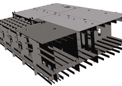
Рис. 1. Результаты трансляции части 3D-модели корпуса
из САПР Tribon в Autodesk Inventor
Специалисты компании CSoft Санкт-Петербург (Бюро ESG) помогли нам транслировать из Tribon в Autodesk Inventor часть корпусной конструкции, состоящую из 800 элементов (рис. 1), а также структуру и наименования, принятые в Tribon. Что особенно важно — при этом была сохранена система отсчета координат и привязок по проекту. За двадцать минут, которые заняла трансляция, мы получили полноценную и качественную сборку объектов корпусных конструкций для дальнейшей работы с ними в среде Autodesk.
Импорт созданных в среде Autodesk Inventor 3D-моделей в Tribon осуществляется при помощи утилиты, обеспечивающей чтение SAT-формата. Без такого импорта не обойтись, когда 3D-модели имеют очень сложную форму и трудны для создания в Tribon.
Autodesk Inventor позволяет создавать реалистичные и очень точные с геометрической точки зрения 3D-модели. В рамках разработки электронных макетов энергетической установки была проведена огромная работа по формированию моделей оборудования, размещенного в машинных отделениях. На основе чертежей, подготовленных в AutoCAD, в среде Autodesk Inventor были созданы полноценные корпусные конструкции (элементы набора, насыщение, фундаменты), произведена трассировка и разводка систем, обслуживающих ГЭУ, систем вентиляции и общекорабельных, проходящих через помещения машинных отделений.
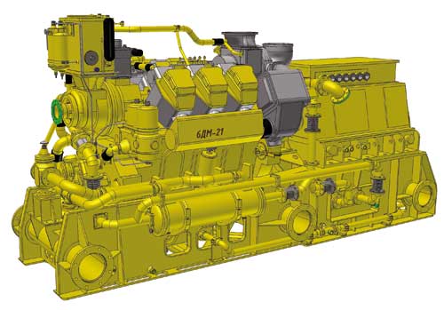
Рис. 2. Судовой дизель-генератор АДГ-630НК
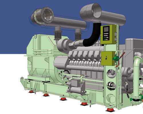
Рис. 3. Дизель-генератор MTU 16V4000
На рис. 2 и 3 представлены 3D-модели дизель-генераторов, которые в кратчайшие сроки были созданы с помощью Autodesk Inventor для электронного макетирования текущих проектов.
Модель дизель-генератора MTU 16V4000 была конвертирована из модели, сформированной в SolidWorks и любезно предоставленной нам немецкой компанией MTU. Модель же судового дизель-генератора АДГ-630НК полностью создана средствами Autodesk Inventor.
На рис. 4 и 5 приведены спроектированные при помощи инструментов Autodesk Inventor элементы трубопроводов систем, находящихся в помещениях машинных отделений. Средствами программы в процессе моделирования был осуществлен анализ пересечения элементов трубопроводов и исправлены выявленные коллизии, что значительно ускорило согласование и выпуск РКД по этим системам.

Рис. 4. Элементы водоотливной системы
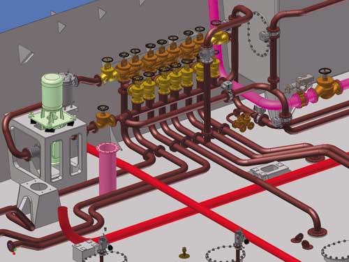
Рис. 5. Элементы топливоперекачивающей системы
В процессе отладки — механизм выпуска рабочей документации с использованием инструментов Autodesk Inventor: чертежи общего расположения создаются на основе макета и транслируются в AutoCAD для дальнейшего оформления.
Наряду с расширением и упорядочением существующей базы 3D-моделей, которая будет использоваться при новом проектировании, и дальнейшей отработкой процедур обмена данными между Autodesk Inventor и Tribon, специалисты ФГУП ЦМКБ «Алмаз» приступили к созданию 3D-моделей машинных отделений по новым заказам для ВМФ РФ.
Таким образом, с появлением Autodesk Inventor процесс проектирования на нашем предприятии претерпел существенные изменения. Назовем лишь некоторые преимущества, ставшие доступными после внедрения этого программного продукта:
• уменьшение сроков выпуска и согласования РКД;
• возможность создания эксплуатационной документации верхних уровней;
• большой выбор инструментов, применимых для судостроительной отрасли;
• простое обучение пользователей AutoCAD работе в Autodesk Inventor (родственный интерфейс, мощная система интерактивной помощи и поддержки);
• широкие возможности импорта-экспорта из других САПР и многое другое.
Эти преимущества были надлежащим образом оценены руководством ФГУП ЦМКБ «Алмаз», которое намерено продолжить плодотворное сотрудничество с компанией CSoft Санкт-Петербург (Бюро ESG). Было принято решение заменить временные лицензии на постоянные, заключен договор на обучение пользователей и техническую поддержку на всех этапах работ.
В заключение хочется подчеркнуть, что внедрение Autodesk Inventor и реализация пилотных проектов осуществлялись совместными усилиями специалистов CSoft Санкт-Петербург (Бюро ESG) и предприятия ФГУП ЦМКБ «Алмаз».
От ФГУП ЦМКБ «Алмаз»:
• заместитель генерального директора — генерального конструктора Марк Давыдович Бройдо;
• начальник 31-го отдела (отдела ГЭУ и систем, обслуживающих ГЭУ) Константин Геннадьевич Голубев;
• начальник 22-го отдела (отдела внедрения САПР Tribon) Алексей Анатольевич Карпов;
• инженер-конструктор I категории (31-й отдел) Евгений Владимирович Маков;
• инженер-конструктор II категории (31-й отдел) Александр Александрович Нортов.
От CSoft Санкт-Петербург (Бюро ESG):
• руководитель отдела САПР Игорь Вячеславович Шептунов.
САПР и графика 11`2006